Section 8.3: Hypothesis Testing Means
Learning Objectives
1.Describe and interpret the Student’s t-distribution.
2.Use the T-distribution to find test statistics and P-Values for hypothesis testing means.
3.Conduct full hypothesis tests for means.
In the last section, we tested hypotheses that were made about qualitative variables put in terms of proportion (or percent) of a population. For example, we tested the claim that the proportion of vaccinated individuals was really 78%, as claimed by the CDC. Vaccination status (vaccinated, or not vaccinated) is a qualitative variable. We were able to consider the qualitative variable as a binomial experiment, interpret the distribution of sample proportions, and under the right circumstances, investigate probabilities to judge claims.
In this section, we will test claims about quantitative variables (numerical sample data) and their means. For example, in section 8.1, we considered the claim that the mean sentence given to Black males in federal courts was longer than for the rest of the population. We used sample data consisting of the sample mean and standard deviation, calculated a Z-score, and found a P-Value from the standard normal distribution. Unfortunately, that approach is not quite right. Because our sample was very large, the result we obtained was reliable. But what if the sample size was smaller? Sadly, under those conditions, a normal distribution does not give us reliable results because of the error in estimating the standard deviation from the sample data. Fortunately, there is a different, but similar distribution, called Student’s t-Distribution that works. We will use it to compute P-Values and test hypotheses for population means.
Student’s T-Distribution
Recall that if we are given a parent distribution with mean and standard deviation , then the distribution of sample means is described in terms of center, variation, and shape as:
•
•
• is normally distributed if either
◦The parent distribution X is normal, or
◦The sample size , or both.
The z-score formula for a sample mean is , which follows a standard normal distribution (mean = 0 and standard deviation = 1).
Now here is the problem. The standard deviation for the distribution of sample means is . Therefore, we need to know the population standard deviation of the original distribution to claim that Z-scores for sample means follow a standard normal curve. But to calculate the population standard deviation we first need to know the population mean . Since we don’t know what it is, we are stuck. We can’t judge the accuracy of a claimed population mean without first knowing the population standard deviation , and we can’t know the population standard deviation unless we first know . Yikes! That’s quite the conundrum!
Fortunately for us, people like beer.
A chemist named William Gossett worked for the Guinness Brewery in Dublin, Ireland in the early 1900’s. His job was to keep the beer Guinness produced consistent throughout the brewing process. Gossett realized that in his statistical analysis, he could not model the distribution of sample means using the normal distribution because the sample sizes were small, and the standard deviations varied too much from sample to sample. He consulted with experts (such as Karl Pearson and Ronald Fisher) and with their help, created a new distribution, which he published under the name “Student.” The Guinness company would not allow him to publish his work using his own name or mentioning beer (they were afraid of losing company secrets to other beer producers and did not wish to lose their advantage in the beer market). Gossett called his distribution the “t” distribution, and it has been called “Student’s t-distribution” ever since. Now, we often call it just the t-distribution, and you will find it under this name in statistical apps or software. In STATBELT, it is the “T-distribution Calculator” under the Calculators menu.
To create the t-distribution, Gosset took the standard normal variable and replaced the population standard deviation with the sample standard deviation, s. This created a new variable
which we say has n – 1 degrees of freedom (explained more below).
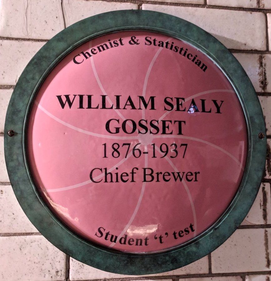
Source: Tim Bates- Wikipedia CC BY-SA 4.0 (opens in a new tab)
Student’s t-distribution
Assume that samples of size n are randomly selected from a population of numerical values, and sample mean and sample standard deviation s are calculated from each sample. If the population is approximately normal, or if , then the distribution
is a t-distribution with n – 1 degrees of freedom.
When using technology, you will sometimes be asked for the degrees of freedom, and other times you will need only the sample size. The technology you use will specify which you need.
The t-distribution looks very similar to a normal distribution, but due to the uncertainty in the standard deviation, it is a little flatter and a little wider. There is a slightly different distribution for every sample size and associated n – 1 degree of freedom. The tails contain a little more area than the standard normal, and the middle contains a little less area. As the sample size increases, the t-distribution will get closer to normal (this is a result of the central limit theorem from section 7.3). That is why the sample size is included in the computation of the t-statistic. See figure 8.11. Observe that the larger the sample size is, the higher the degrees of freedom are, and the closer the t-distribution is to the standard normal curve.
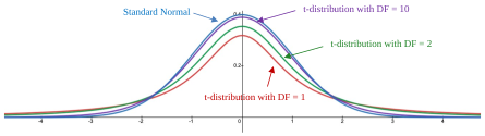
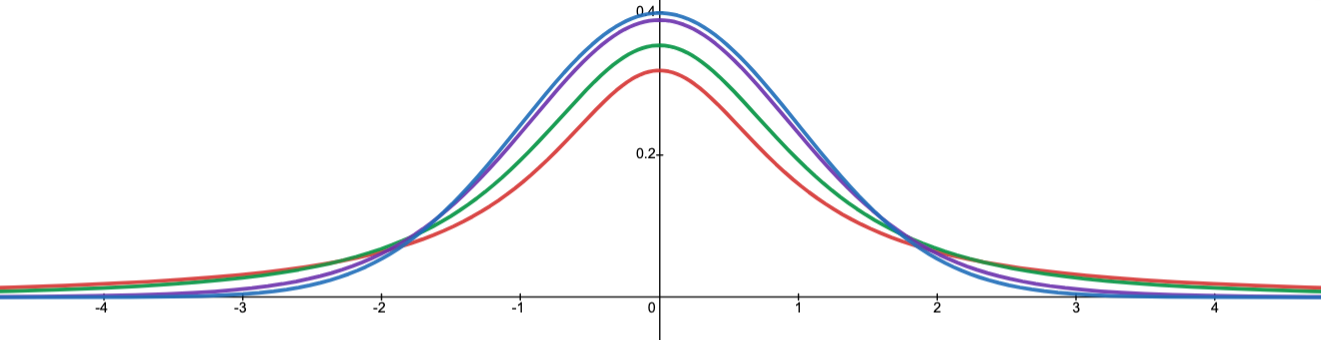
Figure 8.11: Student’s t-distribution for 1, 2, and 10 degrees of freedom, and standard normal distribution.
Degrees of freedom are an odd concept. Why are the degrees of freedom n – 1? The degrees of freedom count how many “independent” pieces of information there are in a sample if we already know the mean. One might think that we need all n data points, but it turns out that we only need n – 1. It is the same reason we divide by n – 1 when we compute the sample standard deviation (section 3.2). Think of this example. If 4 students are offered a choice of 4 different donuts, say 1chocolate, 1 maple, 1 glazed, and 1sprinkled, then the first three students who pick have choices. But the last student has no freedom to choose. Their choice is determined for them. They simply take whatever donut is left. So, there are 4 – 1 = 3 students who are free to choose, one less than the number in the group. The Degrees of freedom in a t-distribution work in a similar way. And because the sample standard deviation is part of the calculation of the t-statistic, it uses n – 1, just like the sample standard deviation.
STATBELT Utility- Probability for Student’s t-Distribution
To use STATBELT Utility to find probability from a t-distribution:
1.Select Calculators → T-distribution Calculator.
2.Type the degrees of freedom DF = n – 1.
3.Under “Find a probability,” choose the inequality you need and type the value or values of t. (The calculator writes T for the variable.)
•Choose “P(T < a)” or “P(T > a)” for one value.
•Choose “P(a < T < b)” to calculate a probability between two values.
4.The probability and a graph appear as soon as you type. There is no button to click.
NOTE: The calculator gives the probability and shows the t-distribution with the probability shaded as area. Click “Open graph in a new window” to see a larger graph.
Example 1: Using Student’s T-Distribution
Assume that a population is normal with an assumed mean . A sample of size n = 64 is taken with sample mean and sample standard deviation s = 18.4.
a)Calculate the test statistic .
b)Identify the degrees of freedom.
c)Find the probability .
Solution:a)To calculate the value of the t-statistic, we will substitute , , , and n = 64.
b)The sample size is n = 64, so there are n – 1 = 64 – 1 = 63 degrees of freedom.
c)To find , open STATBELT Utility and select Calculators → T-distribution Calculator. Type 63 for the degrees of freedom. Under “Find a probability,” choose “P(T < a)” and type -1.174 for the value a. The distribution of the t-variable with 63 degrees of freedom is shown in figure 8.12. .
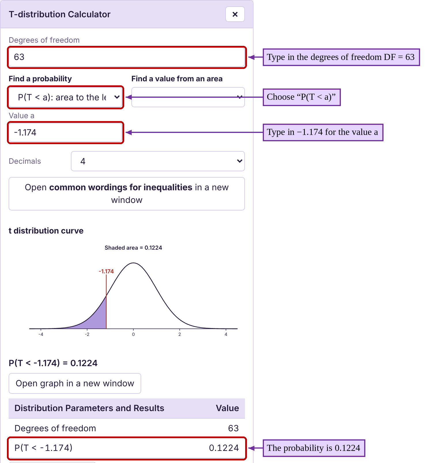
Figure 8.12: Student’s t-distribution with 63 degrees of freedom.
Example 2: Using Student’s T-Distribution
Assume that a population is normal with an assumed mean A sample of size n = 100 is taken with sample mean and sample standard deviation s = 5.6.
a)Calculate the test statistic .
b)Identify the degrees of freedom.
c)Find the probability .
Solution:a)To calculate the value of the t-statistic, we will substitute , , , and n = 100.
b)The sample size is n = 100, so there are n – 1 = 100 – 1 = 99 degrees of freedom.
c)To find , open STATBELT Utility and select Calculators → T-distribution Calculator. Type 99 for the degrees of freedom. Under “Find a probability,” choose “P(T > a)” and type 3.223 for the value a. The distribution of the t-variable with 99 degrees of freedom is shown in figure 8.13. .
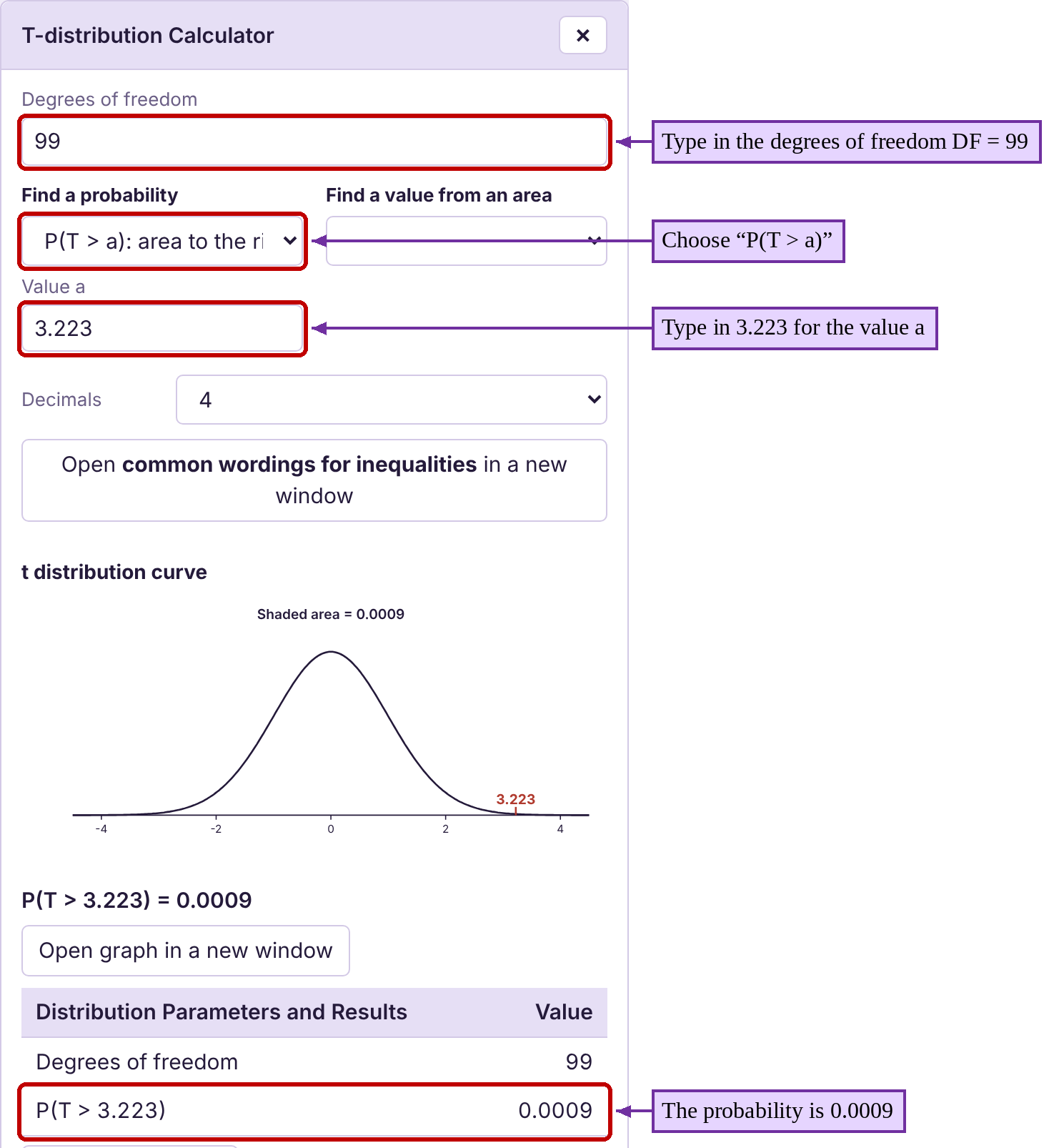
Figure 8.13: Student’s t-distribution with 99 degrees of freedom.

Photo above taken by the author on the Guinness Brewery tour in Dublin, Ireland.
The Process of Hypothesis Testing Means
Now we are ready to test hypotheses regarding means of populations. It is the same process that we used in section 8.2, summarized in the flowchart shown in figure 8.14. In this section, all hypotheses will relate to the mean of a population.
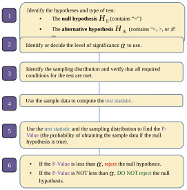
Figure 8.14: The steps of hypothesis testing.
Assume that a claim has been made about the mean of a population. In step 1 we will identify the null and alternative hypotheses. The variable we will use will be , the variable representing the population mean.
Hypothesis Testing Means Details
Step 1:Identify the null and alternative hypotheses. The null hypothesis is . The alternative hypothesis is
• for a left tailed test
• for a right tailed test
•or for a two-tailed test
Step 2:Identify the significance level to use.
Step 3:To conduct a hypothesis test for a mean, we need to check that
•Samples of size n are randomly selected from a population
•The population is approximately normal, or
• and s are calculated from the sample of size n.
Step 4:Calculate the test statistic which follows a t-distribution with n – 1 degrees of freedom. ( is the value assumed true in the null hypothesis.)
Step 5:Calculate the P-Value using the T calculator with n – 1 degrees of freedom. The probability depends on the type of test.
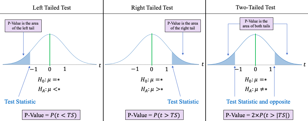
Step 6:If the P-Value is less than the significance level , reject the null hypothesis. If the P-Value is not less than , do not reject the null hypothesis.
Example 3: Mechanics- Hypothesis Testing Means
Assume that a hypothesis test is conducted at the level with the following hypotheses:
The sample data has sample size n = 75 with test statistic t = -1.739. Find the P-Value. Do you reject or fail to reject the null hypothesis at the 0.05 significance level?
Solution:We will apply the six-step process for hypothesis testing a mean.
Step 1:In this problem, we are given the hypotheses, so step 1 is completed for us. This is a left tailed test because the alternative hypothesis is .
Step 2:We are asked to use significance level 0.05.

Step 3:We will assume that the data comes from a simple random sample. The sample size is Since the hypothesis test is about means, the test statistic will follow a t-distribution with n – 1 =
75 – 1 = 74 degrees of freedom.
Step 4:Normally, we would have to compute the test statistic, but it has been calculated for us with t = -1.739.
Step 5:This is a left tail test, so the P-Value is . Open the T-distribution Calculator in STATBELT, or your favorite T-calculator app, type DF = 74, choose “P(T < a)” and type -1.739 for the value a.
The result is P-Value = .
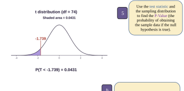
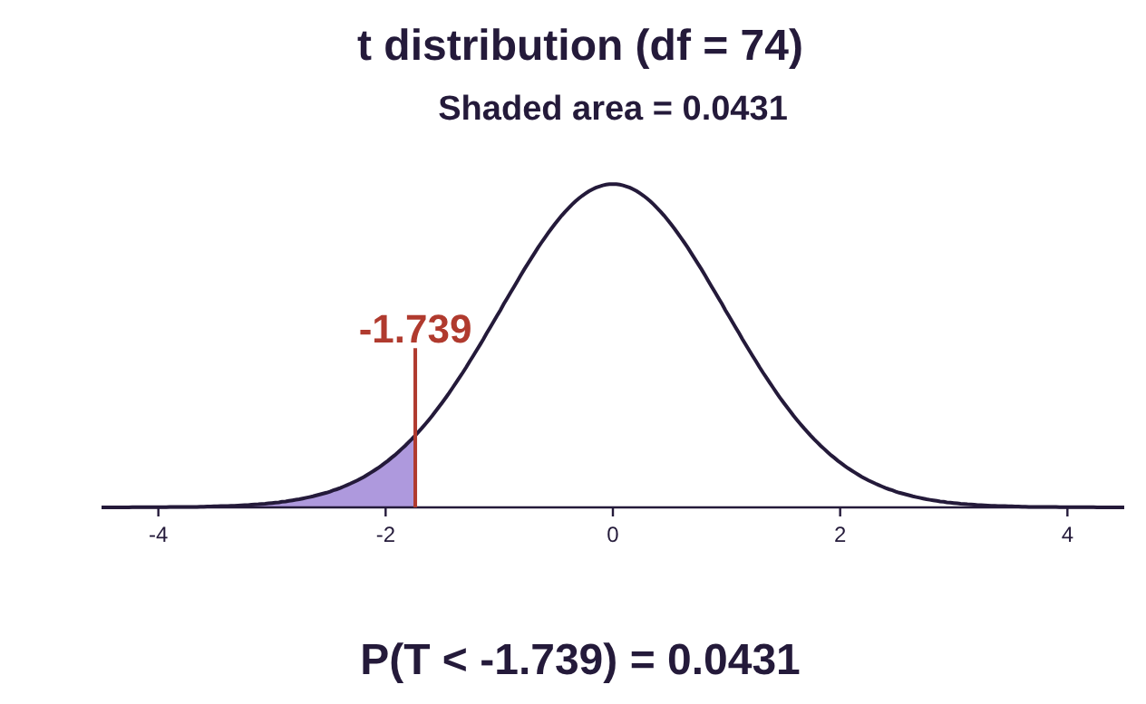
Step 6:Since the P-Value = 0.0431 is less than 0.05, we reject the null hypothesis. The sample data support the claim that the mean is lower than 72.

Example 4: Mechanics- Hypothesis Testing Means
Assume that a hypothesis test is conducted at the level with the following hypotheses:
The sample data has sample size n = 38 with test statistic t = -1.814. Find the P-Value. Do you reject or fail to reject the null hypothesis at the 0.05 significance level?
Solution:We are asked to conduct a hypothesis test for a mean, so we will apply the six-step process.
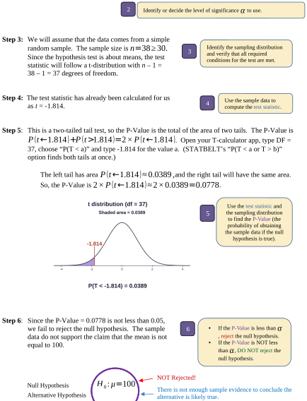
Step 1:In this problem, we are given the hypotheses, so step 1 is completed for us. Since the alternative hypothesis is , this is a two-tailed test.
Step 2:We are asked to use significance level 0.05.
Step 3:We will assume that the data comes from a simple random sample. The sample size is Since the hypothesis test is about means, the test statistic will follow a t-distribution with n – 1 =
38 – 1 = 37 degrees of freedom.
Step 4:The test statistic has already been calculated for us as t = -1.814.
Step 5:This is a two-tailed tail test, so the P-Value is the total of the area of two tails. The P-Value is . Open your T-calculator app, type DF = 37, choose “P(T < a)” and type -1.814 for the value a. (STATBELT’s “P(T < a or T > b)” option finds both tails at once.)
The left tail has area and the right tail will have the same area. So, the P-Value is .
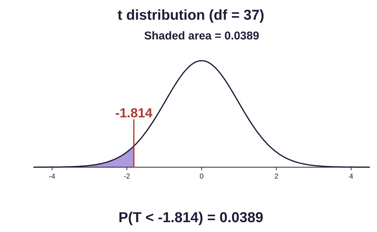
Step 6:Since the P-Value = 0.0778 is not less than 0.05, we fail to reject the null hypothesis. The sample data do not support the claim that the mean is not equal to 100.
Example 5: Mechanics-Hypothesis Testing Means
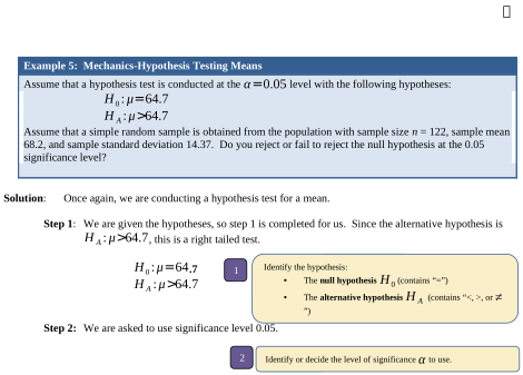
Assume that a hypothesis test is conducted at the level with the following hypotheses:
Assume that a simple random sample is obtained from the population with sample size n = 122, sample mean 68.2, and sample standard deviation 14.37. Do you reject or fail to reject the null hypothesis at the 0.05 significance level?
Solution:Once again, we are conducting a hypothesis test for a mean.
Step 1:We are given the hypotheses, so step 1 is completed for us. Since the alternative hypothesis is , this is a right tailed test.
.7
Step 2:We are asked to use significance level 0.05.
Step 3:We are told that the data comes from a simple random sample. The sample size is Since the hypothesis test is about means, the test statistic will follow a t-distribution with n – 1 =
122 – 1 = 121 degrees of freedom.
Step 4:The test statistic has not been calculated for us as in the last two examples, so we will compute it now.
To calculate the value of the t-statistic, we will substitute , , , and n = 122.

Step 5:As this is a right tailed test, the P-Value is . Use the T calculator with DF = 121, choose “P(T > a)” and type 2.690 for the value a.
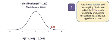
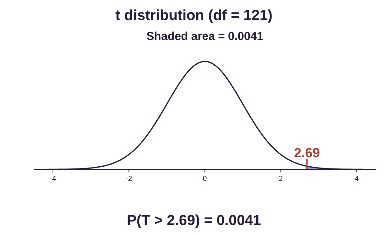
Step 6:The P-Value is approximately 0.0041, which is less than the significance level 0.05. So, we reject the null hypothesis. There is ample evidence to conclude that the alternative hypothesis, that the mean is larger than 64.7, is likely true.

Example 6: Mechanics-Hypothesis Testing Means- Full Process
Assume that a hypothesis test is conducted at the level with the following hypotheses:
A simple random sample has sample size n = 96 with sample mean 1287 and sample standard deviation 342. Test the hypothesis at the 0.05 significance level.
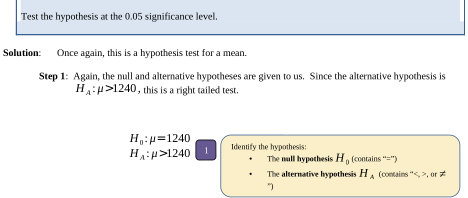
Solution:Once again, this is a hypothesis test for a mean.
Step 1:Again, the null and alternative hypotheses are given to us. Since the alternative hypothesis is this is a right tailed test.
Step 2:We are asked to use significance level 0.05.
Step 3:We are told that the data comes from a simple random sample. The sample size is Since the hypothesis test is about means, the test statistic will follow a t-distribution with n – 1 =
96 – 1 = 95 degrees of freedom.
Step 4:To calculate the value of the t-statistic, we will substitute , , , and n = 96.

Step 5:Since this is a right tailed test, the P-Value is . Use the T calculator with DF = 95, choose “P(T > a)” and type 1.347 for the value a.
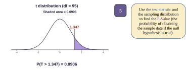
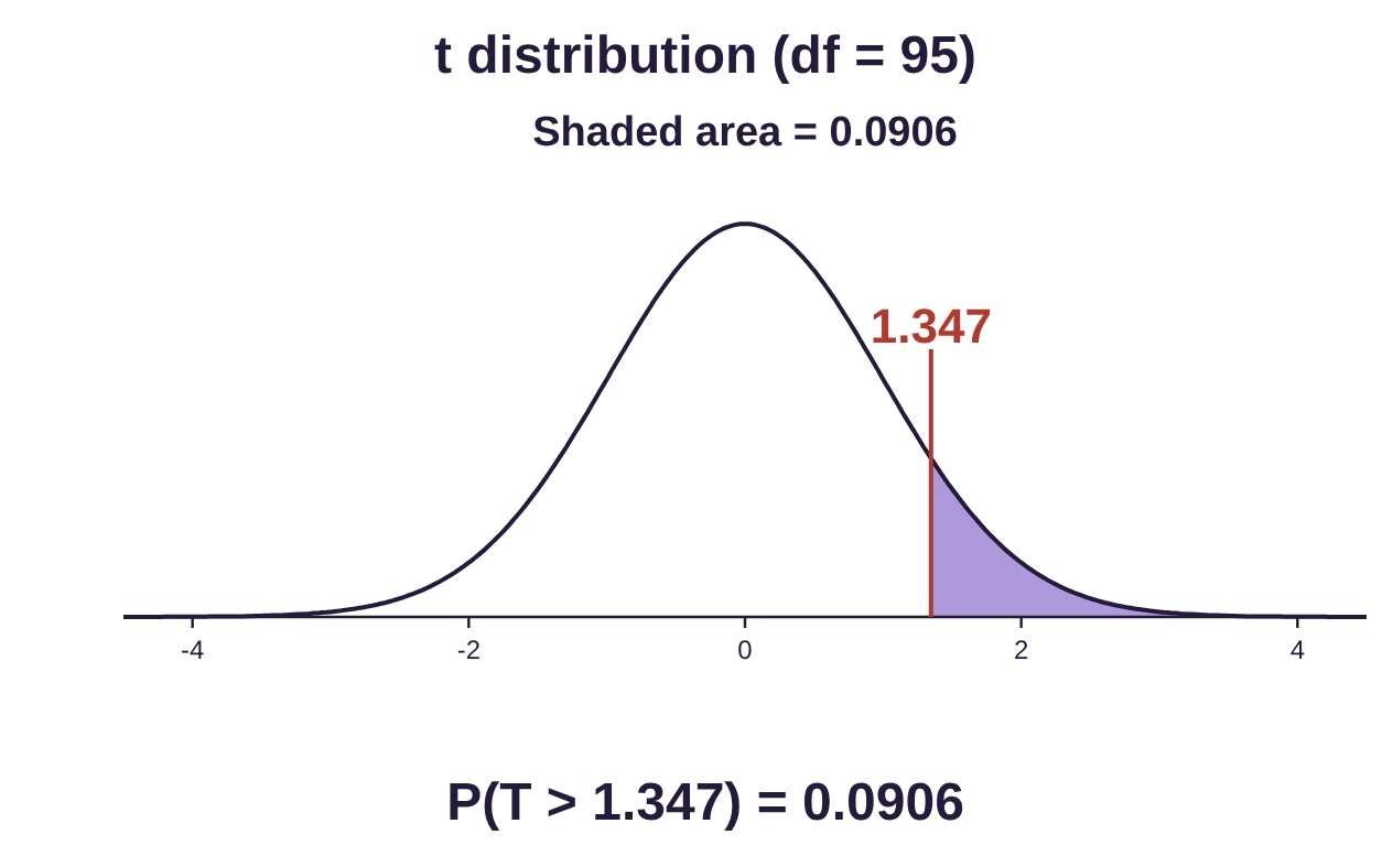
Step 6:The P-Value is approximately 0.0906, which is not less than the significance level 0.05. So, we fail to reject the null hypothesis that the mean is 1240. There is not enough evidence to conclude that the mean is larger than 1240.
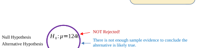

Many technologies, including STATBELT, offer a shortcut that allows us to run the test without computing the test statistic first, as we did in examples 5 and 6. STATBELT and similar apps will ask you to input the hypotheses and the sample mean, standard deviation, and sample size, then will compute the test statistic and P-Value for you. These are commonly called t-tests in technology menus.
STATBELT Utility- Hypothesis Testing Means
To conduct a hypothesis test for a mean using STATBELT Utility and summarized data, follow the path:
Tests → Inference for Means → One sample → Hypothesis test (choose “Column data from the main spreadsheet” if you have a column of raw data).
1.Under “Where is the data?” choose “Summarized data.” Type the sample mean, sample standard deviation, and the sample size n.
2.Type the mean μ from the null hypothesis into “Hypothesized mean μ₀.”
3.Under “Type of test,” choose Left-tailed (<), Right-tailed (>), or Two-tailed (≠).
4.Type the significance level α. The results appear as soon as you type.
The output from STATBELT will include the test statistic, the degrees of freedom, and the P-Value.
Example 7: Hypothesis Testing Means Using STATBELT Utility
In this example, we will use a t-test and let the technology compute the test statistic and P-Value. Assume that a hypothesis test is conducted with the following hypotheses:
A simple random sample has size n = 136 with sample mean 1219 and sample standard deviation 227. Test the claim at the 0.01 significance level.
Solution:Again, this is a hypothesis test for a mean.
Step 1:The null and alternative hypotheses are given to us. Since the alternative hypothesis is
this is a right tailed test.
Step 2:We are asked to use significance level 0.01, not 0.05 like the previous examples!
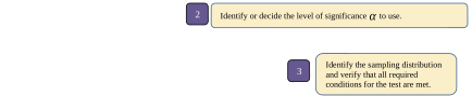
Step 3:We are told that the data comes from a simple random sample with sample size
Since the hypothesis test is about means, the test statistic will follow a t-distribution with n – 1 =
136 – 1 = 135 degrees of freedom.
Steps 4 and 5: Select Tests → Inference for Means → One sample → Hypothesis test.
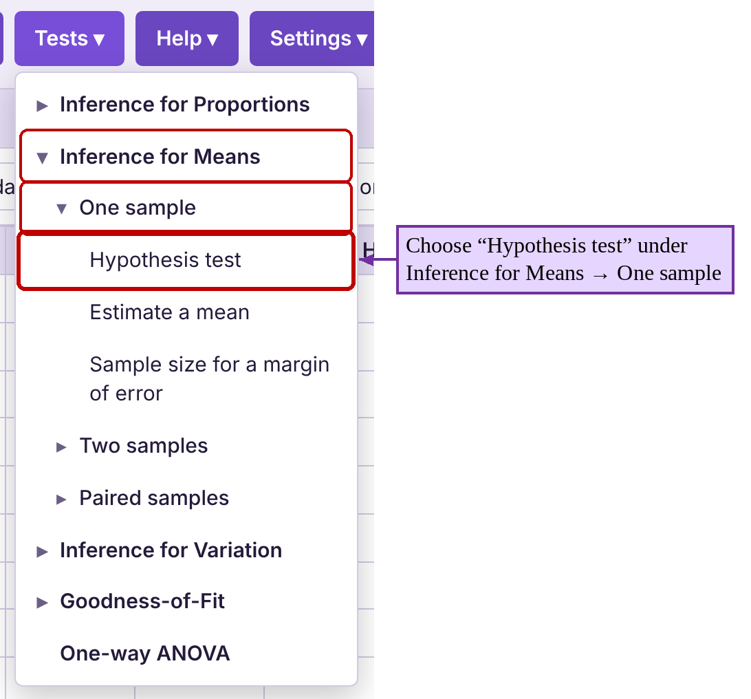
Choose “Summarized data.” Type the sample mean 1219, sample standard deviation 227, and the sample size 136.
Type 1185 for the mean in the null hypothesis and choose “Right-tailed” for a right tailed test. Type 0.01 for the significance level. Click “Open results in a new window” to see the results shown in figure 8.15.
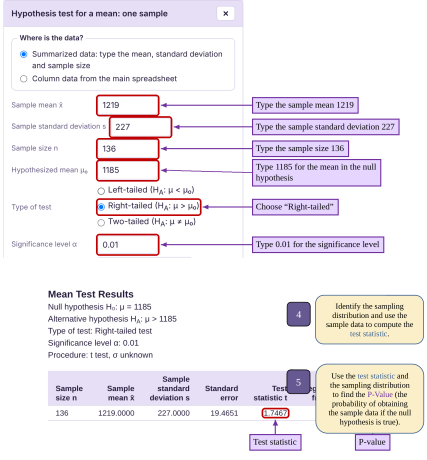
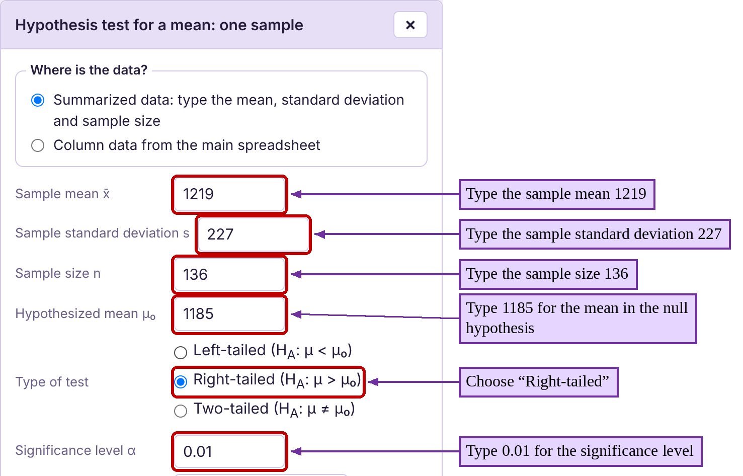
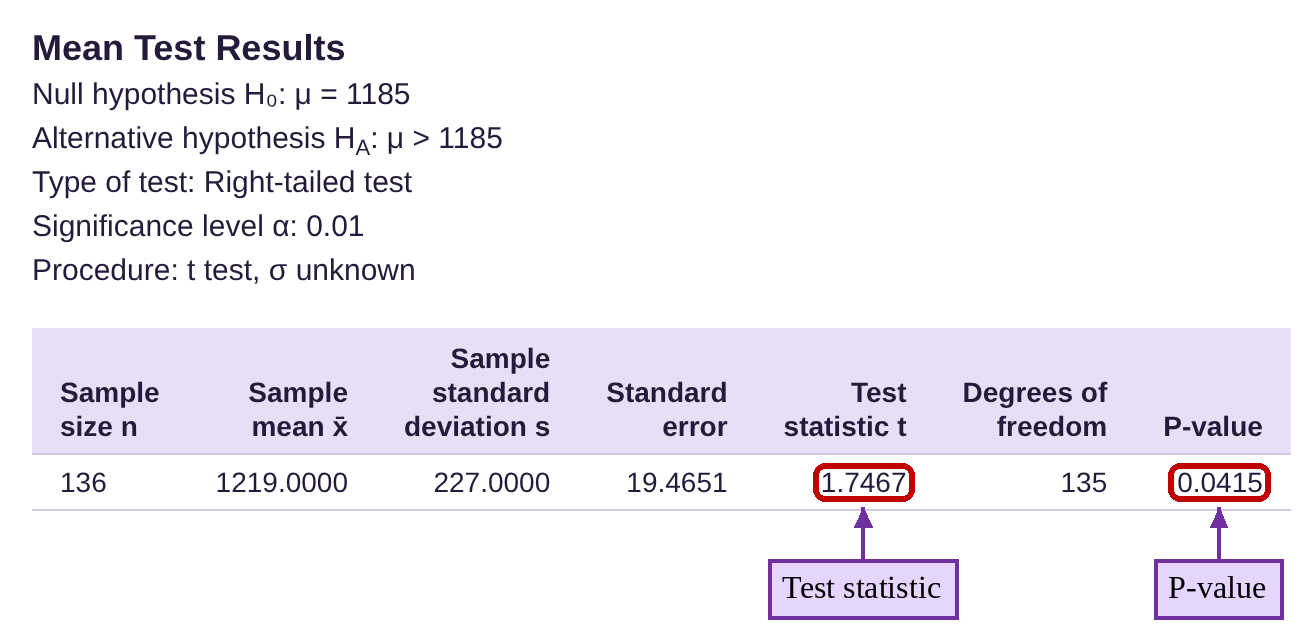
Figure 8.15: STATBELT Utility t-test output.

Step 6:The P-Value is 0.0415, which is not less than the significance level 0.01. So, we fail to reject the null hypothesis that the mean is 1185. There is not enough evidence at the 0.01 significance level to conclude that the mean is larger than 1185.
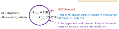

There are two things you should note about example 7. First, the technology computed the test statistic and P-Value for us, which was a fabulous shortcut! Second, even though the P-Value was less than 0.05, we did NOT reject the null hypothesis because for this problem the significance was 0.01. The default level of significance is 5%, but if the consequences of a Type I error are severe, you may choose to use a lower significance level.
Full Hypothesis Tests of Means
We are now ready to test hypotheses with context. We will test the first example twice, once using the six-step process for those using only a probability calculator, and second using a t-test in STATBELT.
Example 8: Hypothesis Testing Means
According to the most recent report from the Student Watch (funded by the National Association of College Stores Foundation) the average cost for course materials (textbooks, electronic subscriptions, etc.) was $456 per course during the 2020-2021 academic year. An independent researcher decided to see if the costs have declined going into the 2022-2023 academic year. They obtain a sample of 48 randomly selected students with a sample mean course materials cost of $339 and standard deviation $207. Test the researcher’s claim at the 0.01 significance level. Have the costs for course materials decreased?
Solution:In context, we are asked if there is enough evidence to conclude that the average (mean) cost has declined. We will use a hypothesis test for a mean to evaluate the claim.
Step 1:We are given the average cost for course materials in 2020-2021 was $456 per course. The word average in this case is referring to the mean. So, the null hypothesis is that the mean is unchanged. The independent researcher believes the cost has declined (is now less than $456) and collects data to try to prove it. This is the alternative hypothesis, making it a left tailed test.

Step 2:We are asked to use significance level 0.01.
Step 3:We are told that the data comes from a random sample with sample size

Photo by Element5 Digital (opens in a new tab) on Unsplash (opens in a new tab)
Since the hypothesis test is about means, the test statistic will follow a t-distribution with n – 1 =
48 – 1 = 47 degrees of freedom.
Step 4:To calculate the value of the t-statistic, we will substitute , , , and n = 48.
Step 5:As this is a left tailed test, the P-Value is . Use the T calculator with DF = 47, choose “P(T < a)” and type -3.916 for the value a.
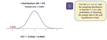
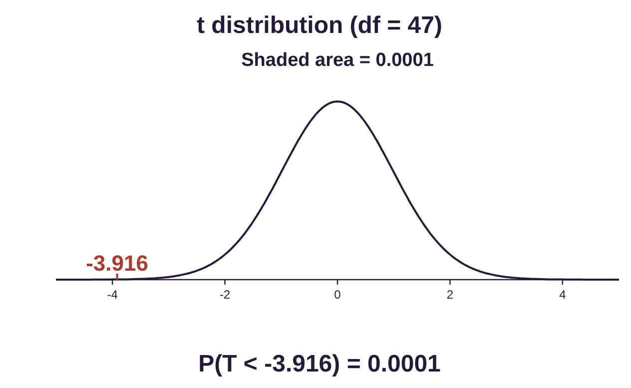
Step 6:The P-Value is approximately 0.0001, which is less than the significance level 0.01. So, we reject the null hypothesis that the mean cost of course materials during the 2022-2023 academic year remains $456. There is enough evidence to conclude that the cost of course materials has decreased. Yay!

Example 9: Hypothesis Testing Means Using STATBELT Utility
Now let’s redo example 8 using the t-test that is built into STATBELT. According to the most recent report from the Student Watch (funded by the National Association of College Stores Foundation) the average cost for course materials (textbooks, electronic subscriptions, etc.) was $456 per course during the 2020-2021 academic year. An independent researcher decided to see if the costs have declined going into the 2022-2023 academic year. They obtain a sample of 48 randomly selected students with a sample mean course materials cost of $339 and standard deviation $207. Test the researcher’s claim at the 0.01 significance level. Have the costs for course materials decreased?
Solution:Steps 1,2 and 3 are identical to example 8.
Step 1:This is a left tailed test for the following hypotheses:
Step 2:We will conduct the hypothesis test using significance 0.01.
Step 3:The data come from a simple random sample with size , so the distribution of sample means is approximately normally distributed, and the test statistic follows a t-distribution with 47 degrees of freedom.
To complete steps 4 and 5 in STATBELT, select Tests → Inference for Means → One sample → Hypothesis test. Choose “Summarized data,” then type the sample mean = 339, sample standard deviation = 207, and sample size = 48. Type 456 for the null hypothesis, choose “Left-tailed,” and type 0.01 for the significance level.
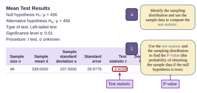
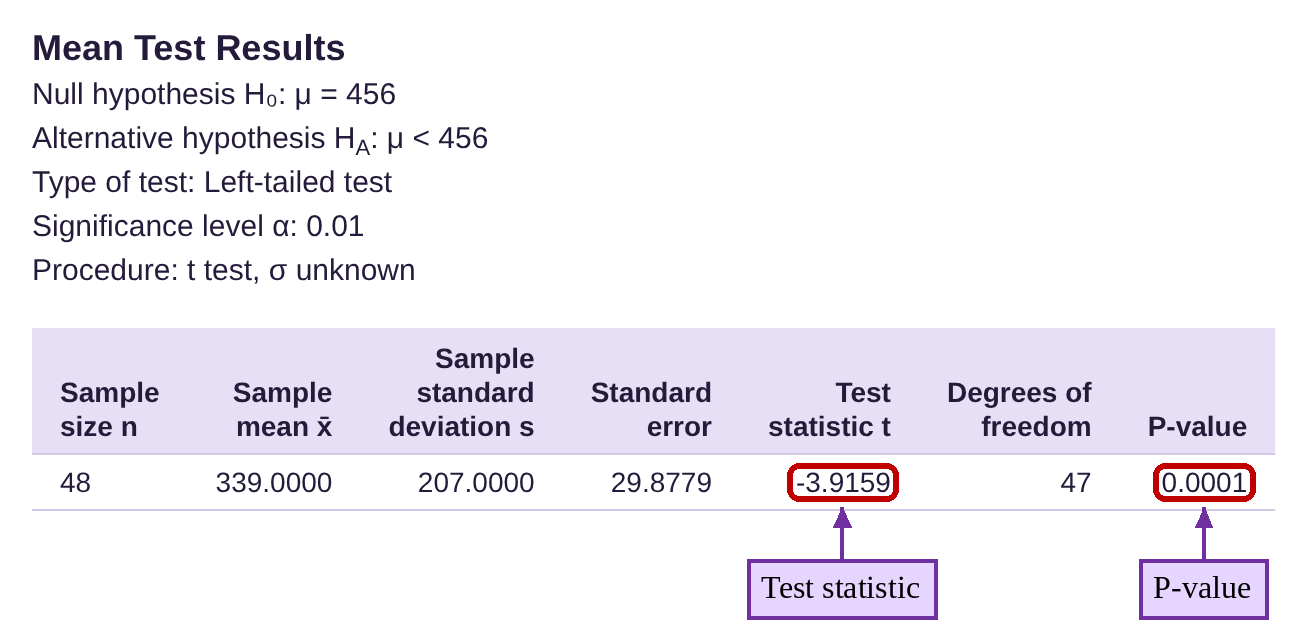
Step 6 is the same as in example 8. The P-Value rounded off at 0.0001, which is less than the significance level 0.01. So, we reach the same conclusion. Notice that STATBELT calculated the test statistic, degrees of freedom, and P-Value for you (the output rounds the P-Value to four decimal places; choose more places under “Decimals” to see more). They are the same as the values that we computed in example 8. Technology offers a shortcut to working out the test statistic and calculating the P-Values by hand!
The flowchart in figure 8.16 summarizes the possible ways to conduct hypothesis tests for means. The left branch shows the six-step process and can be used using any free t-distribution calculator app. The right branch shows the shortcut using STATBELT.
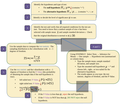
Figure 8.16: Flowchart for testing hypotheses involving means.

Important Points!
Remember: If we compute the test statistic and use the T-calculator to find the P-Value, we use the degrees of freedom to find the probability. But, if we use the t-test with summarized data, we input the sample size n, not the degrees of freedom.
Example 10: Full Hypothesis Test for a Mean
According to the National Student Clearinghouse Research Center (2016 data), the average amount of time it takes students who begin college at a 4-year university to earn a 4-year degree is 5.0 years. A simple random sample of 68 community college students who earned a 4-year degree had a sample mean time of 5.7 years with sample standard deviation 1.82 years. Test the claim that it takes community college transfer students longer than students who start at a university to earn a 4-year degree using significance level 0.05.

Photo by Naassom Azevedo (opens in a new tab) on Unsplash (opens in a new tab)
Solution:We will conduct a hypothesis test using STATBELT with context.
Step 1:We are given that it takes students at a university 5.0 years, on average, to earn their degree. The null hypothesis is that there is no change, and that community college transfer students take the same number of years to complete their degree. The alternative hypothesis is that it takes them longer.
Since the alternative hypothesis is , this is a right tailed test.
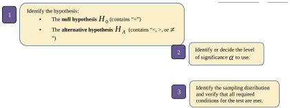
Step 2:We are asked to use significance level 0.05.
Step 3:We are told that the data comes from a simple random sample with sample size
Since the hypothesis test is about means, the test statistic will follow a t-distribution with n – 1 =
68 – 1 = 67 degrees of freedom.
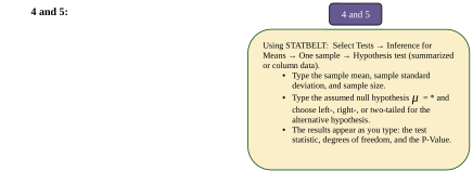
Steps 4 and 5: These two steps are completed by STATBELT. We don’t know the shape of the distribution of the parent population, but we can use the t-distribution because the sample size is n = 68 .
Select Tests → Inference for Means → One sample → Hypothesis test and choose “Summarized data.” Type 5.7 for the mean, 1.82 for the sample standard deviation, and 68 for the sample size. Type 5.0 for the mean given in the null hypothesis. Since this is a right tailed test, choose “Right-tailed.”
The output gives us the sample mean, which we already know, the degrees of freedom equal to 67, the test statistic t = 3.172 and the P-Value = 0.0011.
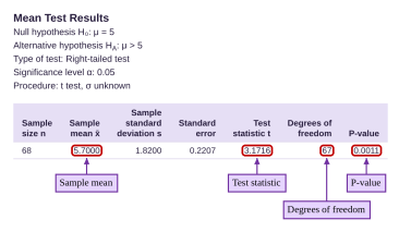
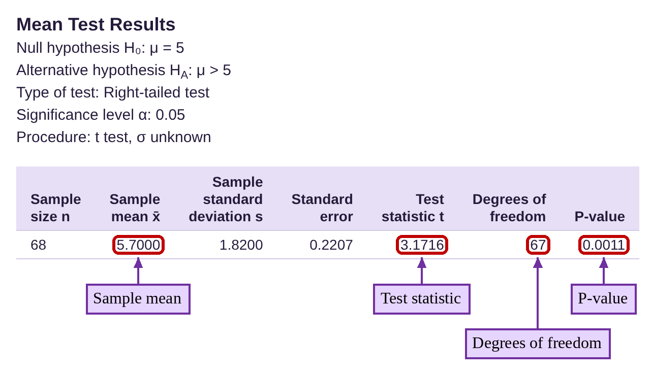
Step 6:Since the P-value = 0.0011 is less than significance , we reject the null hypothesis. There is statistical evidence to conclude that it takes community college transfer students longer to earn their 4-year degree. (But the difference is less than one year, and they save two years of high tuition!)

The final example of this section covers how to conduct a hypothesis test for a mean with raw data. Using STATBELT or another software package you can manage this easily. If you are using a calculator or calculator app, you may have to summarize the data yourself first, then follow the process we have been using. Some apps will allow you to type in the data manually, but that is likely more work than summarizing it yourself first. The best option is to use technology to conduct the test.
STATBELT Utility- Hypothesis Testing Means for Raw Data
To conduct a hypothesis test for a mean using STATBELT Utility and raw data, follow the path:
Tests → Inference for Means → One sample → Hypothesis test.
1.Under “Where is the data?” choose “Column data from the main spreadsheet,” then choose the column that contains the data.
2.Type the mean from the null hypothesis into “Hypothesized mean μ₀.”
3.Under “Type of test,” choose Left-tailed (<), Right-tailed (>), or Two-tailed (≠).
4.Type the significance level α. The results appear as soon as you type.
The output from STATBELT will include the sample mean, the test statistic, and the P-Value, all computed for you!
Example 11: Hypothesis Testing Means from Raw Data
According to a 2017 study conducted by Inside Higher Education, the average high school grade point average at that time was 3.3. A random sample of grade point averages from 48 high school and college students are shown in Table 3. We will test two claims.
1.A student advocacy group believes the claimed grade point average is too high. Test the claim that the mean grade point average of high school students is less than 3.3 using significance level 0.05.
2.A college professor believes that high school grade point averages have been inflated, and that college grade point averages are lower than high school grade point averages. Test the claim that college grade point averages are lower than 3.3 using 0.05 level of significance. You can open the GPA data (opens in a new tab) in STATBELT (download CSV).
Table 3: High School and College Grade Point Averages | |||||||
|---|---|---|---|---|---|---|---|
HS GPA | College GPA | HS GPA | College GPA | HS GPA | College GPA | HS GPA | College GPA |
3.87 | 3.89 | 2.26 | 1.92 | 3.72 | 2.7 | 2.1 | 2.04 |
4 | 3.9 | 3.27 | 3.1 | 2.33 | 3.05 | 2.48 | 2.7 |
2.87 | 2 | 3.11 | 2.9 | 2.93 | 2.33 | 3.74 | 4.06 |
2.99 | 3 | 1.83 | 2 | 3.66 | 3 | 1.49 | 2.23 |
3.22 | 2.83 | 3.84 | 3.43 | 3.49 | 2.4 | 1.89 | 2 |
3.32 | 2.67 | 4 | 4 | 3.44 | 3 | 3.31 | 3 |
2.67 | 2.38 | 3.43 | 3 | 2.49 | 2.25 | 4 | 3.7 |
4 | 3.83 | 3.31 | 3.3 | 2.7 | 2.9 | 3.75 | 2.64 |
3.54 | 3.5 | 2.97 | 3.2 | 3.95 | 3.33 | 3.5 | 3 |
2.63 | 2.6 | 4 | 3.7 | 3.72 | 3.9 | 2.07 | 2.67 |
2.62 | 2.54 | 2.12 | 2.9 | 4 | 3.9 | 3.42 | 3.2 |
4 | 3 | 3.03 | 3 | 4 | 3.54 | 4 | 3.92 |
Solution:The first claim is made about high school students. The claim is that high school grade point averages are lower than 3.3, which was the claim made by Inside Higher Education.

Step 1:The null hypothesis is that the mean high school grade point average is 3.3. The alternative is that it is less than 3.3. Since the alternative hypothesis is , this is a left tailed test.

Step 2:We are asked to use significance level

Step 3:We are told that the data comes from a random sample with sample size We don’t know the sample mean and sample standard deviation, but they can be computed using STATBELT.
Since the hypothesis test is about means, the test statistic will follow a t-distribution with n – 1 = 48 – 1 = 47 degrees of freedom.
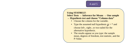
Steps 4 and 5: These two steps are completed by STATBELT. We don’t know the shape of the distribution of the parent population, but we can use the t-distribution because the sample size is n = 48 .
Open the GPA data in STATBELT Utility with the link in the example. Then select Tests → Inference for Means → One sample → Hypothesis test.
Choose “Column data from the main spreadsheet” and the column “HS GPA.” Type 3.3 for the mean from the null hypothesis and choose “Left-tailed” for a left tailed test.
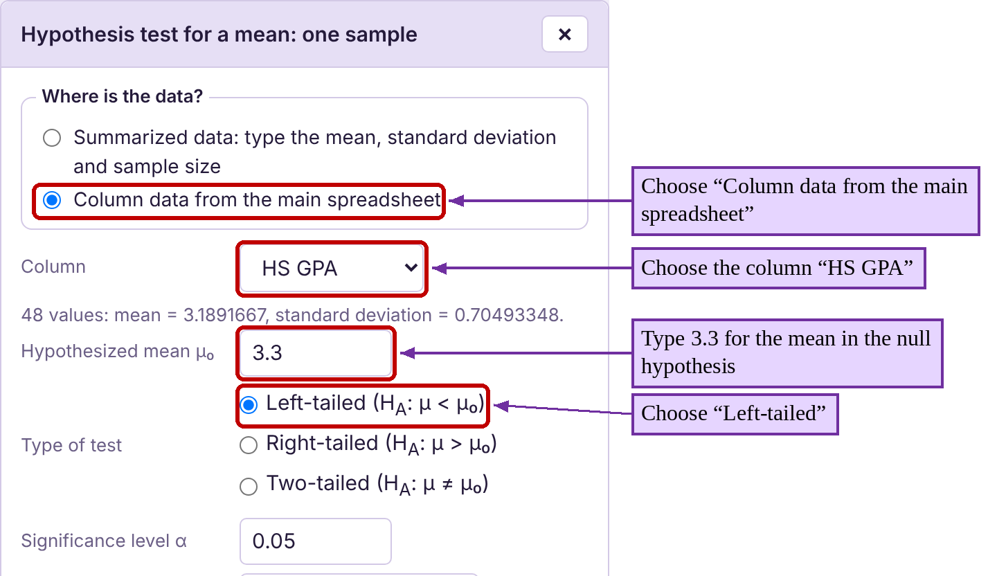
The output gives us the sample mean of high school graduates . The degrees of freedom are listed as 47, and the test statistic is -1.089. The P-Value has been calculated as 0.1408.
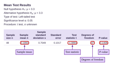
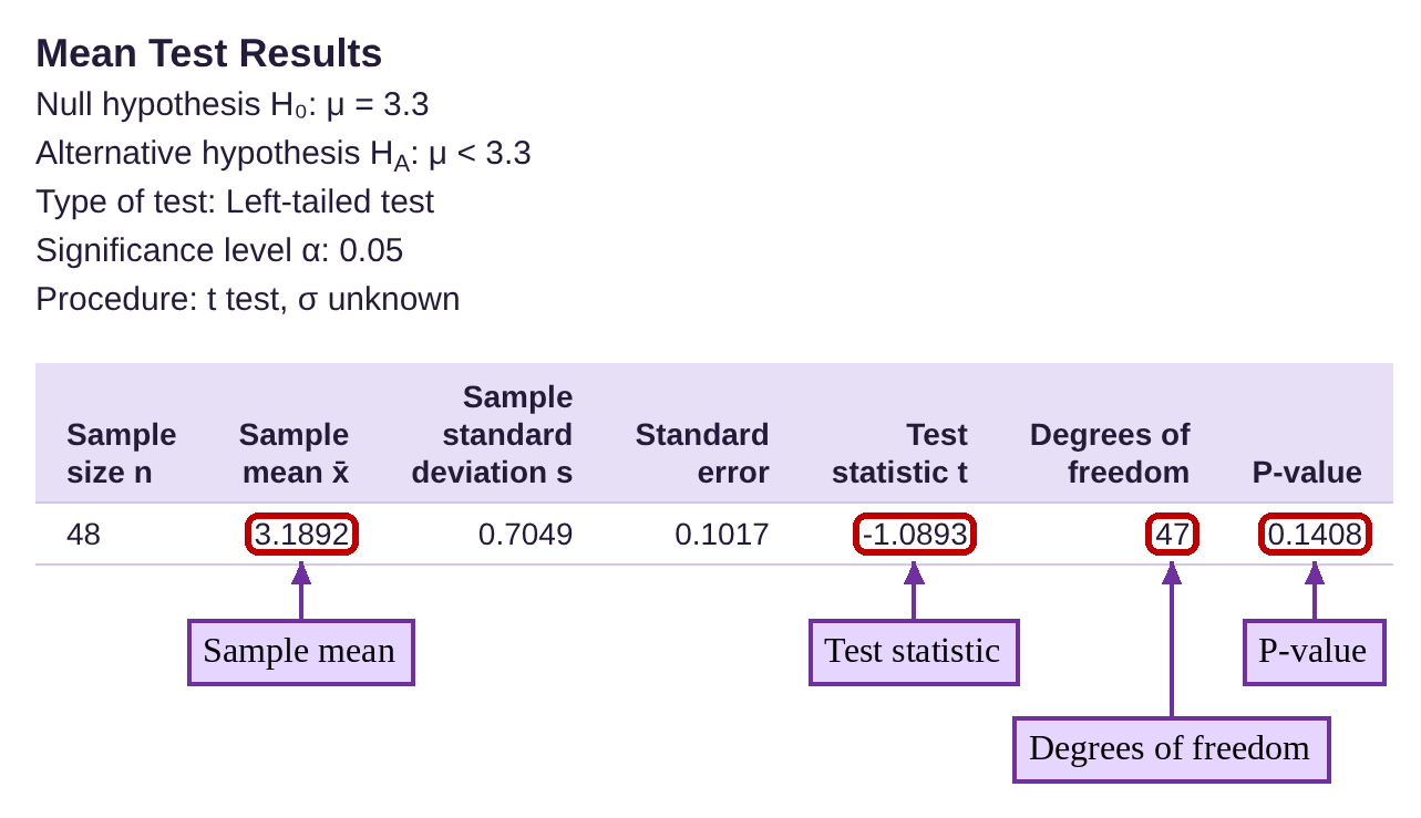
Step 6:Since the P-value = 0.1408 is not less than , we fail to reject the null hypothesis. There is no statistical evidence to conclude that the mean high school grade point average is less than 3.3.

In context, the claim made by Inside Higher education appears reasonable. The second claim that we will test is whether college grade point averages are less than 3.3.

Step 1:The null hypothesis is that the mean college grade point average is the same as high school grade point averages, or 3.3. The alternative is that it is less than 3.3. Again, this is a left tailed test because the alternative hypothesis is .

Step 2:We are asked to use significance 0.05.
Step 3:We have already established that we can use the t-distribution because the data come from a simple random sample with sample size n = 48 .
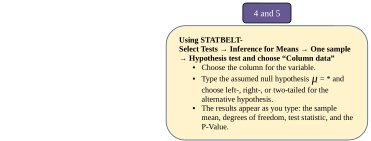
Steps 4 and 5: Once again, we select Tests → Inference for Means → One sample → Hypothesis test.
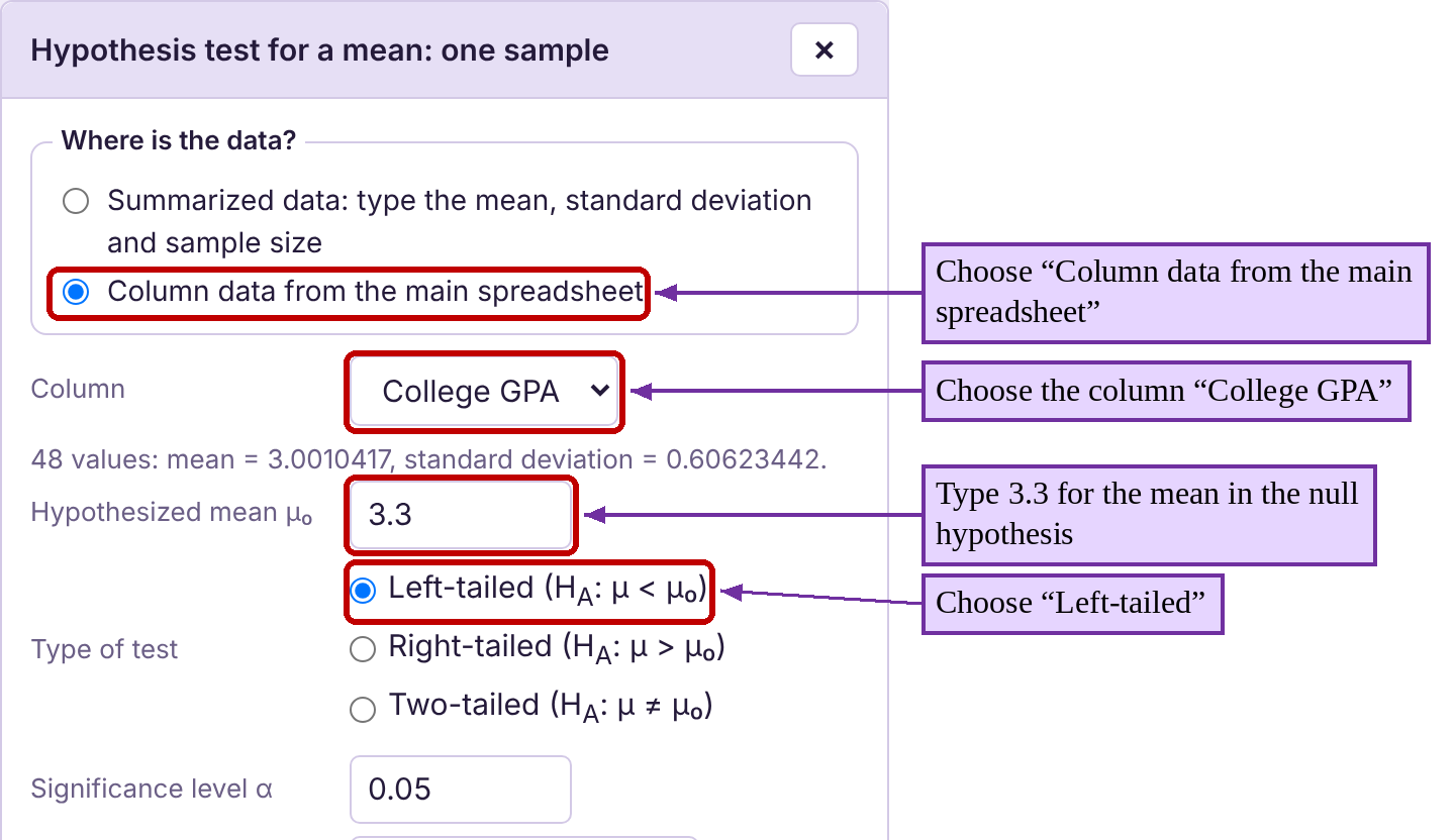
Choose the column “College GPA” this time, type 3.3 for the mean from the null hypothesis, and choose “Left-tailed” for a left tailed test.
The output gives us the sample mean of college grade point averages . The degrees of freedom are listed as 47, and the test statistic is -3.417. The P-Value has been calculated as 0.0007.
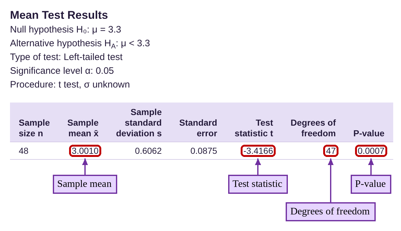

Photo by Felipe Gregate (opens in a new tab) on Unsplash (opens in a new tab)
Step 6:Since the P-value = 0.0007 is less than , we reject the null hypothesis. There is statistical evidence to conclude that the mean college grade point average is less than 3.3.

In context, the claim that the mean high school grade point average is less than 3.3 could not be supported with this data. However, we could conclusively show that the mean college grade point average is lower than 3.3. This supports the idea that it may be easier to obtain better grades in high school than in college.
Finally, what does it mean to be “approximately normal?” Sometimes, data that are mound shaped but not exactly normal may be good enough for the procedures we want to use. In other cases, the procedure may be very sensitive to the normality assumption and give unreliable results if the data are not very close to normal or even precisely normal. The procedures we present in chapters 8, 9, and 10 will work even if the data are not “exactly normal.” In statistics, we say that the procedures are robust. We think of a robust process as one that is flexible and dependable even when the data are not exactly normal. But some procedures that will be discussed in chapter 11 are very sensitive to the assumption that the data come from a normal population. These procedures are not robust! We must be very careful to ensure that the data are normal when we interpret results from those procedures.
Definition 1
A robust statistical process is one that gives reliable results when the data are approximately normal. A statistical process that requires data to be normal and is unreliable when the data are not precisely normal is not robust. All procedures in chapter 8, 9, and 10 are robust.