Section 8.2: Hypothesis Testing Proportions
Learning Objectives
1.Describe the logic of hypothesis testing proportions.
2.Compute test statistics and P-Values for hypothesis testing proportions.
3.Conduct full hypothesis tests for proportions.
The Logic of Hypothesis Testing Proportions
Recall the intuitive idea of hypothesis testing shown in figure 8.6. In this section, we will test claims made about population proportions. These claims are made regarding qualitative variables, or the proportion or percent of a population with a qualitative characteristic.
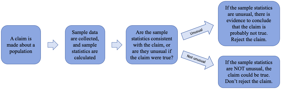
Figure 8.6: The intuitive logic of hypothesis testing.
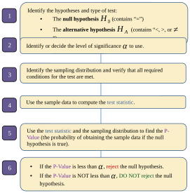
Figure 8.7: The steps of hypothesis testing.
Figure 8.7 shows the steps of hypothesis testing proportions, which is the topic of section 8.2. In this section, all claims we test will be made regarding a population proportion, p.
Hypothesis Testing Proportions Details
Assume that a hypothesis test for a proportion is conducted.
Step 1:Identify the null hypothesis and the alternative hypothesis.
The null hypothesis is
The alternative hypothesis is
) for a left tailed test | a right tailed test | for a two tailed test
Step 2: Identify the significance level .
Step 3:The test requires that a simple random sample of size n is selected with x successes, the conditions for a binomial experiment are met, and . If all are true, then the sampling distribution is normal.
Step 4:If the sampling distribution is normal, the test statistic follows a standard normal distribution (Z- distribution). Calculate the test statistic as the Z-score of the sample proportion:
Test Statistic:
Where , and standard deviation
Step 5:Calculate the P-Value using the standard normal calculator (mean = 0 and standard deviation = 1). The probability depends on the type of test.
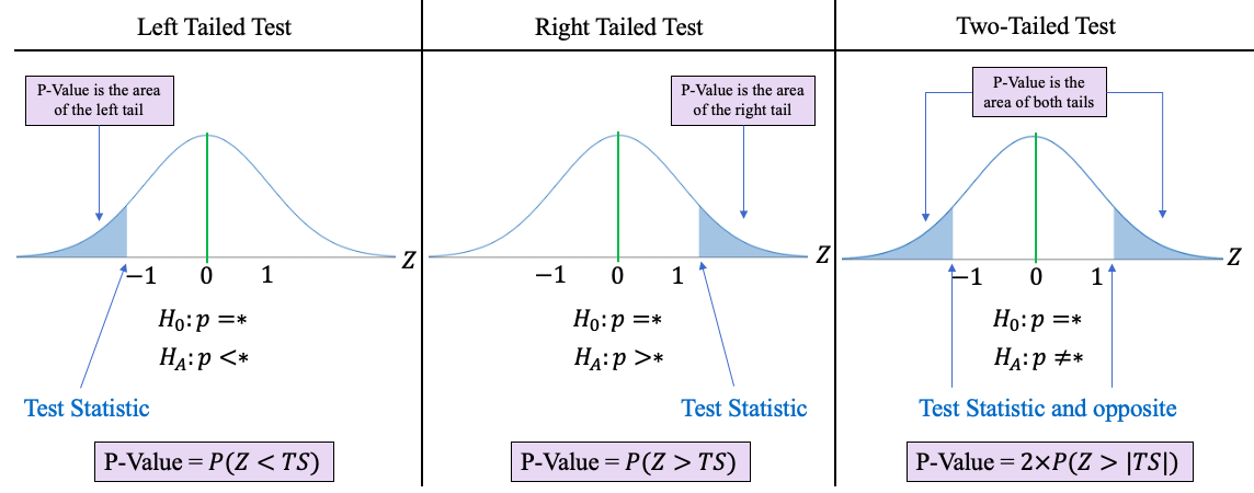
Step 6:If the P-Value is less than the significance level , reject the null hypothesis. If the P-Value is not less than , do not reject the null hypothesis.
Example 1: Hypothesis Testing Proportions Mechanics (Left Tailed Test)
Assume that a hypothesis test is conducted at the level with the following hypotheses:
A simple random sample of size n = 144 has 64 successes. Assume the simple random sample follows the conditions for binomial experiment. Follow the six-step process to complete the hypothesis test.
Solution:In this problem, we are asked to conduct the hypothesis test for a proportion.
Step 1:The null and alternative hypotheses are given. This is a left tailed test.
Step 2:We are told to use significance level .
Step 3:We have a simple random sample with n = 144 and x = 64. We will assume that the conditions of a binomial experiment are met. We need to check that .
Since , the distribution of sampling proportions will have an approximately normal distribution.
Step 4:To compute the test statistic, we need to know the sample proportion and the standard deviation.
The sample proportion is .
The distribution of sample proportions has n = 144 and p = 0.48, which is assumed from the null hypothesis.
The standard deviation is calculated as follows:
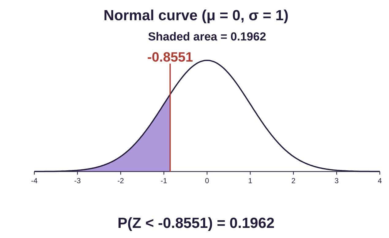
The test statistic is . Substituting , , and , we find the z-score to be 1. So, the sample proportion falls about 0.8551 standard deviations below the mean, if the population proportion is truly 0.48.
Step 5:Since this is a left tailed test, the P-Value is . Using a standard normal calculator (mean = 0 and standard deviation =1), we find .
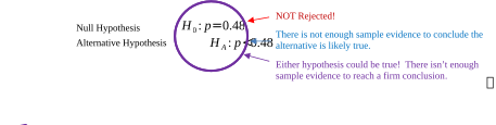
Step 6:Since the P-Value is NOT less than the significance level , this sample data is not unusual if the null hypothesis is true. So, we fail to reject the null hypothesis that the population proportion is p = 0.48, or 48%. The population proportion could be 48%, or it could be lower.

Important Points!
Remember:
•Only reject the null hypothesis when the P-Value is small!
•You never reject the alternative hypothesis, only the null hypothesis!
•Failing to reject the null hypothesis means either hypothesis could be true!
Example 2: Hypothesis Testing Proportions Mechanics (Two-Tailed Test)
Assume that a hypothesis test is conducted at the level with the following hypotheses:
A simple random sample with sample size n = 576 has 438 successes. Assume the simple random sample follows the conditions for binomial experiment. Follow the six-step process to complete the hypothesis test.
Solution:We are asked to conduct a hypothesis test for a proportion.
Step 1:The null and alternative hypotheses are given. This is a two tailed test.
Step 2:We are told to use significance level .
Step 3:We have a simple random sample with n = 576 and X = 438. We assume that the conditions of a binomial experiment are met. We need to check that .
Since , the distribution of sampling proportions will have an approximately normal distribution.
Step 4:To compute the test statistic, we need to know the sample proportion and the standard deviation.
The sample proportion is . This sample proportion is higher than the assumed population proportion of 72%. But is it different enough to reject the null hypothesis? Let’s find out!
The distribution of sample proportions has n = 576 and p = 0.72, which is assumed from the null hypothesis.
The standard deviation is
The test statistic is . Substituting , , and , we find the z-score to be . So, the sample proportion falls a little more than two standard deviations above the mean, if the population proportion is truly 0.72.
Step 5:Since this is a two-tailed test, the null hypothesis will be rejected if either the sample data has a mean that is far below what is expected, or if the sample data has a mean that is far above what is expected. In other words, the P-value is the area of both tails, and the null hypothesis will be rejected if the test statistic is far into the left tail, or far into the right tail. That means that the P-Value is which is Due to symmetry, this is twice the area of either one of the tails.
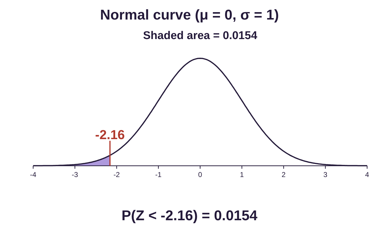
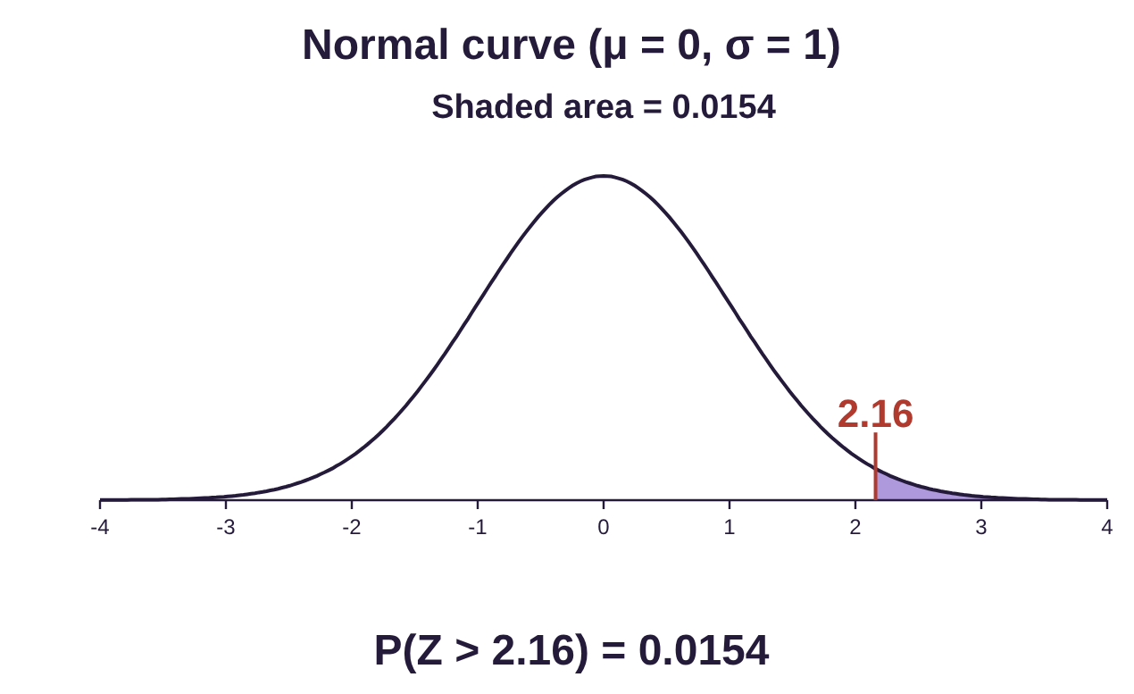
Using a standard normal calculator), we find
P-Value = , or
P-Value = .
Step 6:Since the P-Value = 0.0308 is less than the significance level , the sample data are unusual if the population proportion is really 72%. So, we reject the null hypothesis that the population proportion is p = 0.72. Statistical evidence supports the alternative hypothesis, that the proportion is not equal to 72%.

 Tip!
Two tailed tests are not as common as left and right tailed tests. When conducting a two- tailed test, if the test statistic is positive, use P-Value = .
If the test statistic is negative, use P-Value =.
Some technologies, such as STATBELT Utility, statistical software packages, and many probability apps, allow you the option to conduct a hypothesis test without first computing the test statistic. STATBELT and these apps will ask you to input the hypotheses and the sample data, then will compute the test statistic and P-Value for you. This is a shortcut when compared to the first two examples. But, if you only have access to a probability calculator, you can still complete the work by finding the test statistic first.
STATBELT Utility- Hypothesis Testing Proportions
To conduct a hypothesis test for a proportion using STATBELT Utility and summarized data, follow the path:
Tests → Inference for Proportions → One sample → Hypothesis test.
1.Under “Where is the data?” choose “Summarized data.” Type the number of successes x and the number of trials (the sample size n).
2.Type the proportion p from the null hypothesis into “Hypothesized proportion p₀.”
3.Under “Type of test,” choose Left-tailed (<), Right-tailed (>), or Two-tailed (≠) for the alternative hypothesis.
4.Type the significance level α. The results appear as soon as you type. There is no button to click.
The output from STATBELT will include the sample proportion, the test statistic, and the P-Value. Click “Open results in a new window” for a copy you can save.
Example 3: Hypothesis Testing Proportions Using STATBELT Utility
We will use STATBELT Utility to complete example 1. Assume that a hypothesis test is conducted at the level with the following hypotheses:
The sample data has sample size n = 144 with 64 successes. Use STATBELT Utility (or another app) to complete the hypothesis test.
Solution:The first three steps are identical to example 1.
Step 1:We are given hypotheses for the left tailed test. Step 2: We will use significance level .
Step 3:We checked that , so the distribution of sampling proportions is approximately normal.
Steps 4 and 5: These two steps are completed by STATBELT. Select Tests → Inference for Proportions → One sample → Hypothesis test.
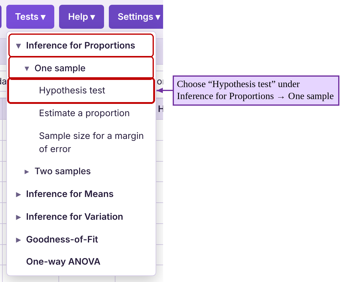
Choose “Summarized data.” Type 64 for the number of successes and 144 for the number of trials. Type 0.48 for the proportion in the null hypothesis, and choose “Left-tailed” under “Type of test” for a left tailed test. The results appear as you type. Click “Open results in a new window” to see the output shown in figure 8.8.
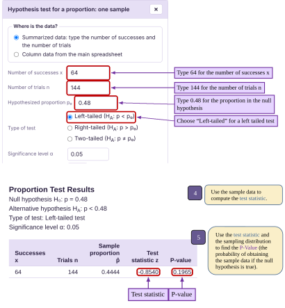
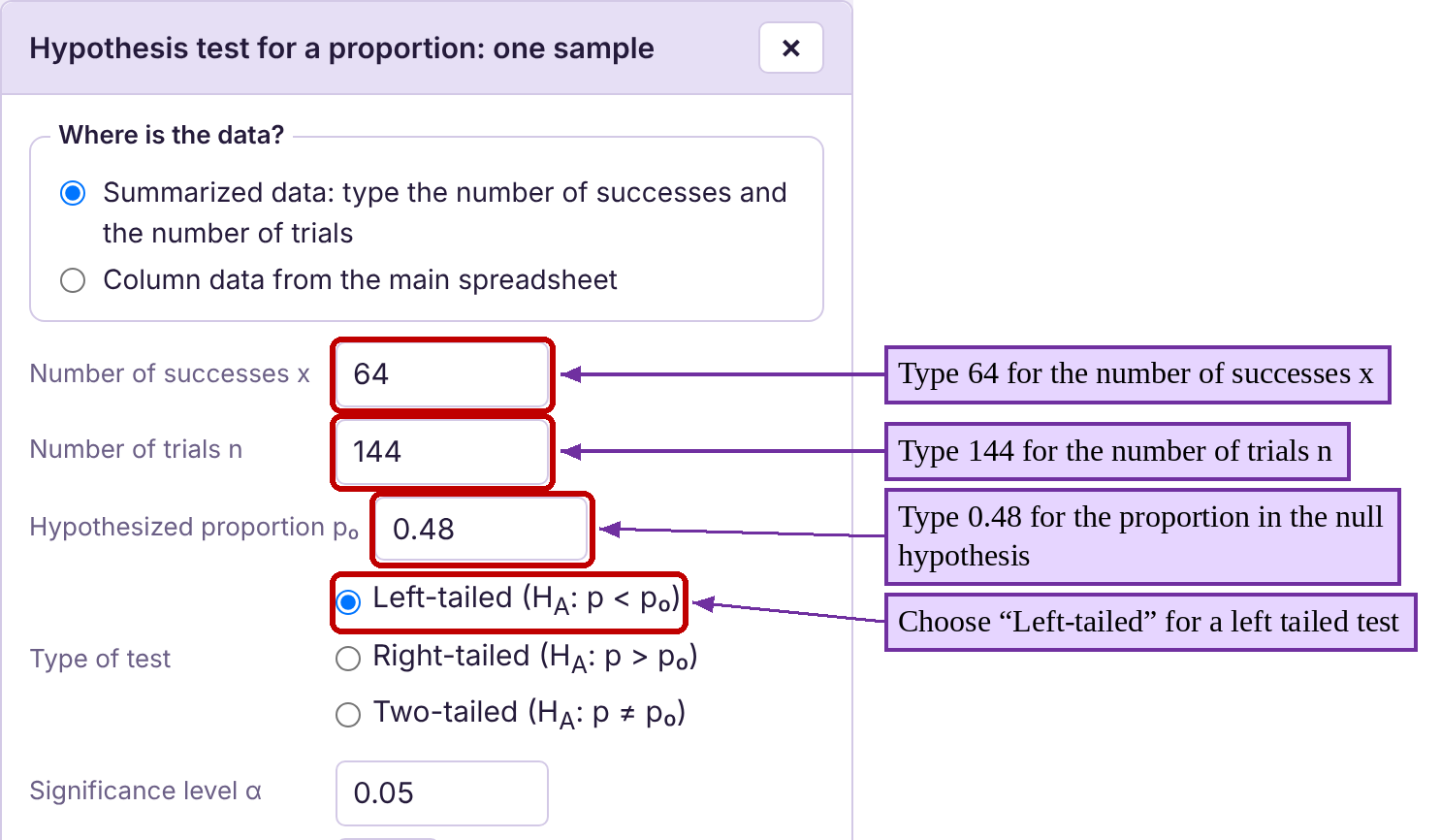
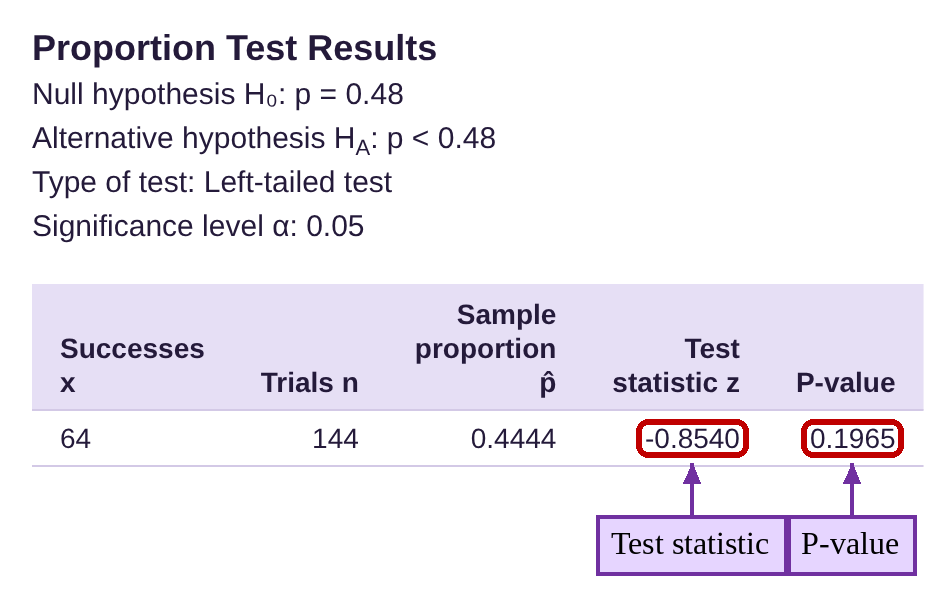
Figure 8.8: STATBELT Utility output for a hypothesis test for a proportion.
The sample proportion is 0.4444, as we calculated in example 1. The test statistic is called “Test statistic z” in the output, and it is -0.8540, which is slightly different from what we calculated due to rounding.
When we calculated the test statistic in example 1, we rounded the sample proportion and the standard deviation, which resulted in a small difference. We found the P-Value to be 0.1962, while STATBELT, using more decimal places, calculated it at 0.1965. They are very close!
Step 6:Since the P-value = 0.1965 is not smaller than , we fail to reject the null hypothesis. There is not enough evidence to conclude that the population proportion is less than 48%. This was the same conclusion reached in example 1, except that we did not need to compute the standard deviation of the sampling distribution of sample proportions to then calculate the test statistic. Technology proved to be a great shortcut!
Example 4: Hypothesis Testing Proportions Using STATBELT Utility
Use STATBELT Utility to conduct the hypothesis test from example 2. Assume that a hypothesis test is conducted at the level with the following hypotheses:
The sample data has sample size n = 576 with 438 successes.
Solution:The first three steps are identical to example 2.
Step 1:The hypotheses for the two-tailed test are: Step 2: We will use significance level .
Step 3:We checked that , so the distribution of sampling proportions is approximately normal.
Steps 4 and 5: These two steps are completed by STATBELT. Select Tests → Inference for Proportions → One sample → Hypothesis test.
Choose “Summarized data.” Type 438 for the number of successes and 576 for the number of trials. Type 0.72 for the proportion in the null hypothesis, and choose “Two-tailed” under “Type of test.” Then click “Open results in a new window.” The output is shown in figure 8.9.
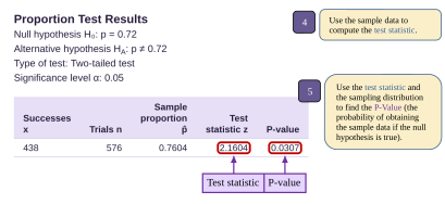
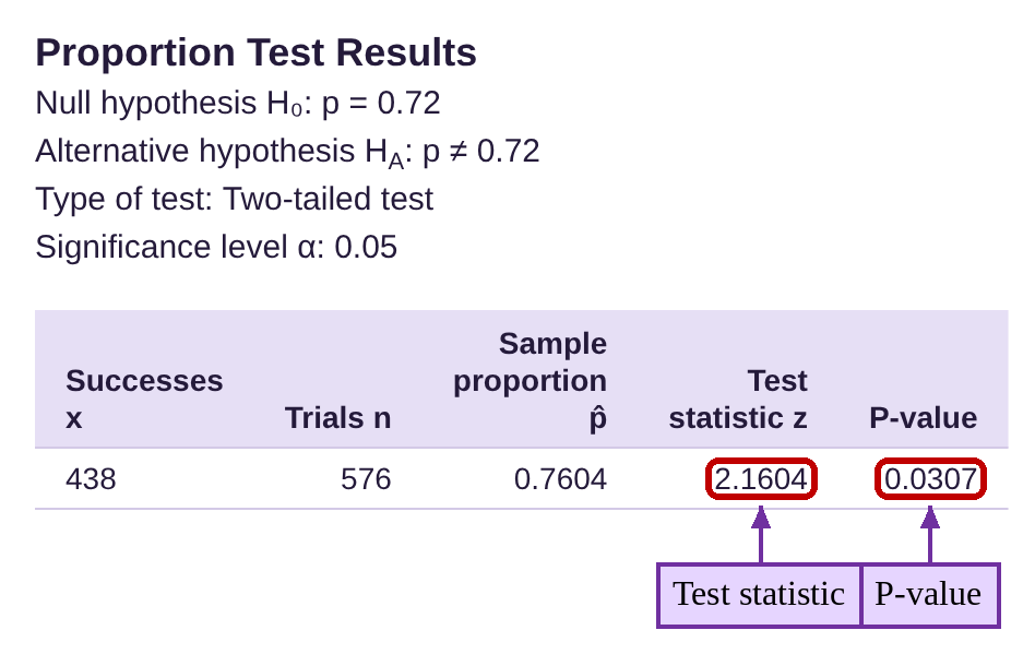
Figure 8.9: STATBELT Utility output for a hypothesis test for a proportion.
The sample proportion is 0.7604 as we calculated in example 2. The test statistic is 2.1604, which rounds to 2.160, just as we calculated previously.
The P-Value is 0.0307, which is close to what we calculated using rounded figures. Note that we did not need to double the area of a tail. STATBELT did that for us and reported the correct P-Value!

Step 6:Since the P-value = 0.0307 is less than , we reject the null hypothesis. There is statistical evidence to conclude that the population proportion is not equal to 72%. This is the same result we reached in example 2.
Full Hypothesis Tests of Proportions
Next, we will put the entire process together using technology. From this point on, we will use STATBELT and its option to type in the summarized data to find the sample proportion, test statistic, and P-Value. However, if you only have access to Desmos, or a free probability distribution calculator, you can still find the test statistic first, then get the P-Value using the probability calculator. Don’t forget to double the area of the tail if you follow that path and conduct a two-tailed test. Figure 8.10 is a revised flowchart for conducting a hypothesis test for proportions by (the left branch) first finding the sample proportion, the test statistic, and the P-Value, and (the right branch) using STATBELT or a more advanced statistics app.
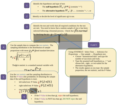
Figure 8.10: Flowchart for hypothesis testing proportions.
Example 5: Full Hypothesis Test for a Proportion
According to the National Pet Owners Survey conducted by the American Pet Products Association in 2019-2020, 38.4% of U.S. households own a dog. A small “dog-friendly” town’s city council believes their town has a greater proportion of dog-owners. They collect a sample of n = 2482 residents with 993 that own dogs. Can the city council conclude that their town has more dog owners than the U.S. average? Use 0.05 significance.

Photo by Lauren McConachie (opens in a new tab) on Unsplash (opens in a new tab)
Solution:In this case we are to test the claim that the proportion of dog owners in the town is higher than the U.S. average.
Step 1:We are given the fact that 38.4% of U.S. households own a dog, so this is what we will assume to be true. The “dog-friendly” town council thinks the percent is higher in their town. Since the null hypothesis is always assumed “=”, the null hypothesis is that the proportion is p = 0.384 (as a decimal), and the alternative is that p > 0.384. This is a right tailed test.

Step 2:We are instructed to use significance level .

Step 3:We will assume that the sample was randomly selected, and that the process adheres to the requirements for a binomial experiment. We need to make sure that the distribution of the sample proportions is normally distributed by verifying that , using n = 2482 and p = 0.384.
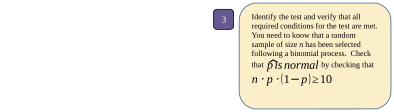
Since , the distribution of sampling proportions will have an approximately normal distribution.
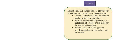
Steps 4 and 5: These two steps are completed by STATBELT. Select Tests → Inference for Proportions → One sample → Hypothesis test and choose “Summarized data.” Type 993 for the number of successes and 2482 for the number of trials. Type 0.384 for p₀, the proportion in the null hypothesis. Since this is a right tailed test, choose “Right-tailed.”
The output gives us the sample proportion of dog owners , with test statistic = 1.647, and P-Value = 0.0498.
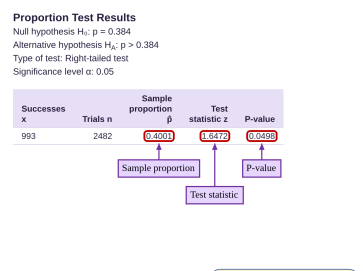
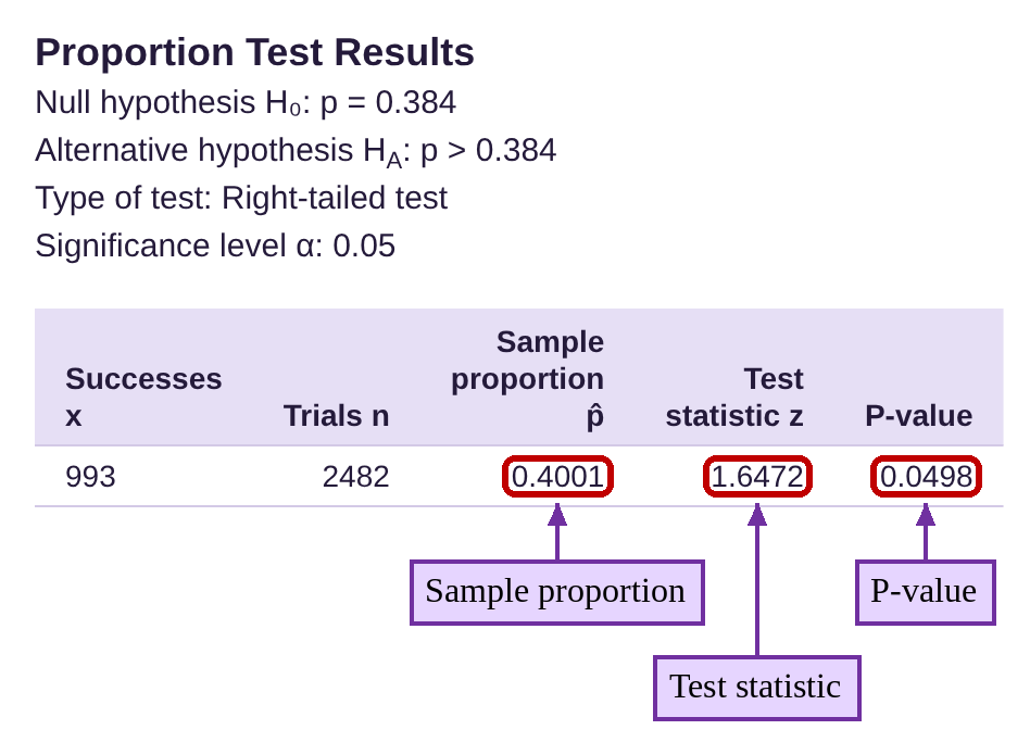
Step 6:Since the P-value = 0.0498 is less than significance , we reject the null hypothesis. In context, there is statistical evidence to conclude that the proportion of dog owners in the town is greater than 38.4%.

Example 6: Full Hypothesis Test for a Proportion
According to the Institute for Health Metrics and Evaluation (IHME), approximately 82% of the U.S. population has been infected with COVID-19 at least once as of July 2022. Assume that 387 residents of Richmond, CA, are randomly selected and 329 had been infected. Can we conclude that Richmond, CA, has had more COVID-19 infections? Use 0.05 significance for the hypothesis test.

Photo by Fusion Medical Animation (opens in a new tab) on Unsplash (opens in a new tab)
Solution:In this problem we are asked to use a hypothesis test to determine if there is a higher proportion of COVID-19 infections in Richmond, CA, than in the U.S.
Step 1:We are given the fact that 82% of the U.S. population has been infected with COVID-19, so this is what we will assume to be true. The question asks if the proportion in Richmond is higher, so the null hypothesis is p = 0.82, and the alternative is that p > 0.82. This is a right tailed test.

Step 2:We are instructed to use significance level .

Step 3:The sample was randomly selected, and we will assume the process adheres to the requirements for a binomial experiment. To verify that the distribution of the sample proportions is normally distributed, we check that , using n = 387 and p = 0.82.
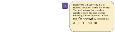
Since , the distribution of sampling proportions will have an approximately normal distribution.
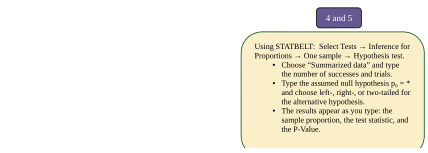
Steps 4 and 5: These two steps are completed by STATBELT.
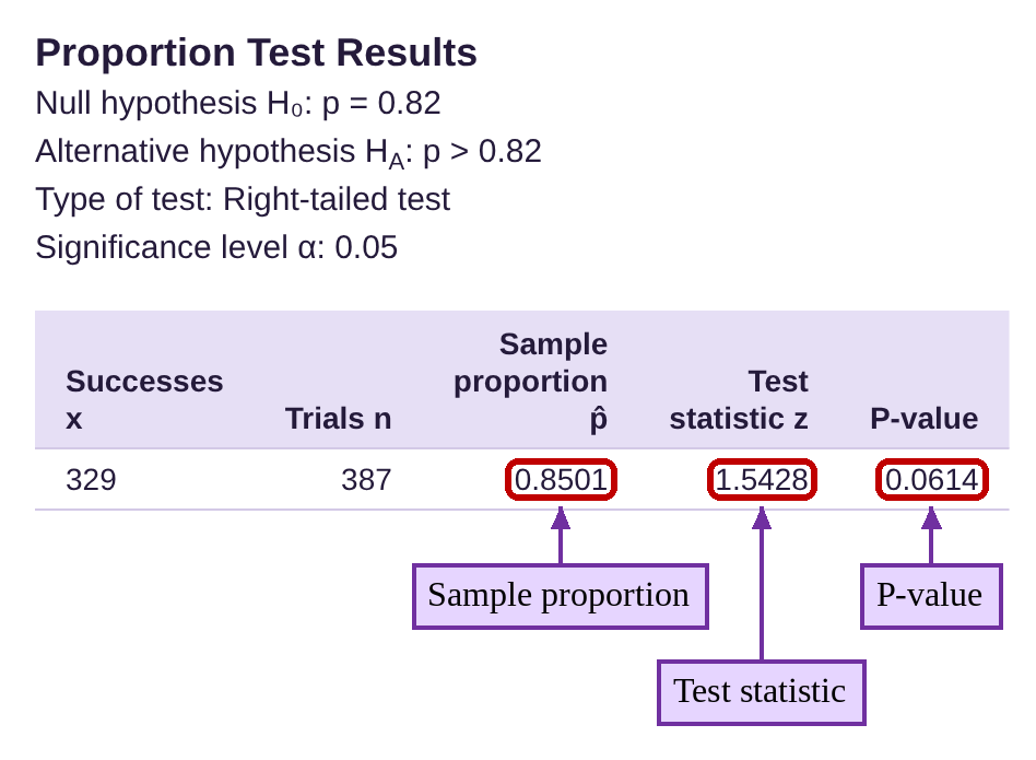
Select Tests → Inference for Proportions → One sample → Hypothesis test and choose “Summarized data.” Type 329 for the number of successes and 387 for the number of trials. Type 0.82 for p₀, the proportion in the null hypothesis. Since this is a right tailed test, choose “Right-tailed.”
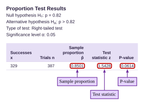
The output gives us the sample proportion of Richmond residents who had COVID-19 as , or about 85%. The test statistic is = 1.543, and P-Value = 0.0614.
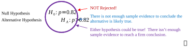
Step 6:Since the P-value = 0.0614 is not less than
, we fail to reject the null hypothesis. There is not enough statistical evidence to conclude that the proportion of Richmond residents infected with COVID-19 is greater than the rest of the U.S. population.
Example 7: High School Graduates and College
According to the National Center for Educational Statistics, 66% of high school graduates immediately enrolled in college in 2019. A researcher believes that the rate of direct enrollment has changed. They collect a random sample of 1039 high school graduates from 2021 of which 645 graduates immediately enrolled in college. Is this enough evidence to conclude that the rate is no longer 66%? Test at the 0.01 significance level.
Solution:Here we are asked to test whether the proportion of students who directly enroll in college has changed.
Step 1:We are given the fact that 66% of high school graduates immediately enrolled in college in 2019. The question asks if the proportion has changed, meaning that it is not equal to 66%. So, the null hypothesis is p = 0.66, and the alternative is that . This is a two tailed test.

Step 2:We are instructed to use significance level .

Step 3:We are told that the sample was randomly selected. Once again, the process appears to be a binomial experiment. To make sure that the distribution of sample proportions is normally distributed, check that , using n = 1039 and p = 0.66
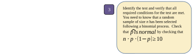
Since , the distribution of sampling proportions will have an approximately normal distribution.
Steps 4 and 5:
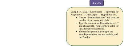
Select Tests → Inference for Proportions → One sample → Hypothesis test and choose “Summarized data.” Type 645 for the number of successes and 1039 for the number of trials. Type 0.66 for p₀, the proportion in the null hypothesis. Since this is a two-tailed test, choose “Two-tailed,” and type 0.01 for the significance level.
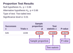
The output gives us the sample proportion of direct enrollment as , or about 62%. The test statistic is -2.668, and P-Value = 0.0076.
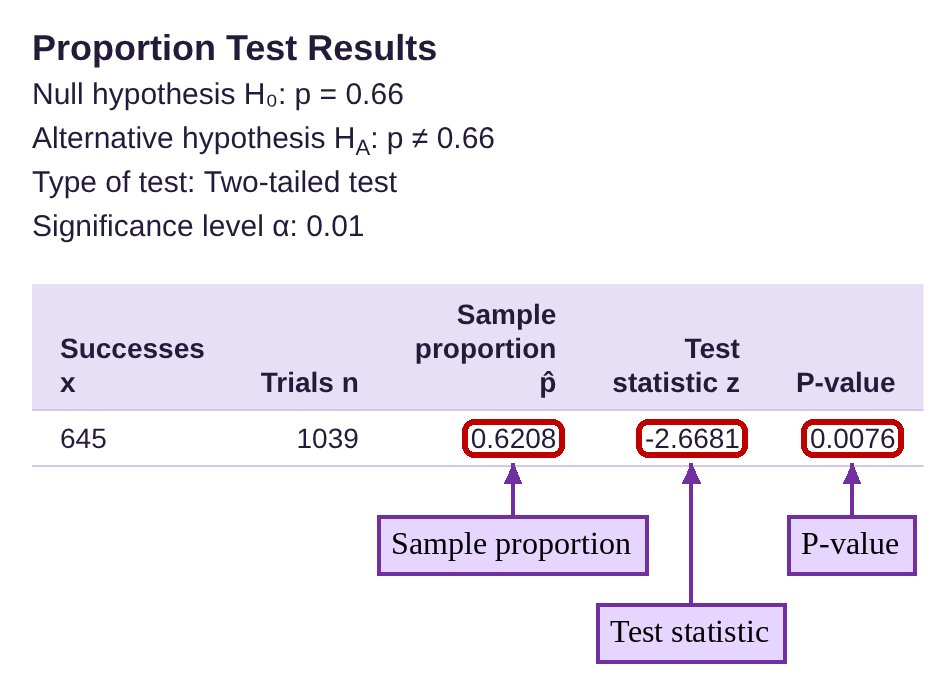
Step 6:Since the P-value = 0.0076 is less than
, we reject the null hypothesis.
There is statistical evidence to conclude that the proportion of students who enrolled directly in college is no longer 66%. Since the sample proportion is about 62%, it appears that the proportion has declined.

The final example of this section covers how to conduct a hypothesis test for proportions with raw data. Using STATBELT or another software package you can manage this easily. If you are using a calculator or calculator app, you may have to summarize the data yourself first, then follow the process we have been using. Some apps will allow you to type in the data manually, but that is likely more work than summarizing it yourself first. The best option is to use technology to conduct the test.
STATBELT Utility- Hypothesis Testing Proportions for Raw Data
To conduct a hypothesis test for a proportion using STATBELT Utility and raw data, follow the path:
Tests → Inference for Proportions → One sample → Hypothesis test.
1.Under “Where is the data?” choose “Column data from the main spreadsheet,” then choose the column that contains the data.
2.Under “Count as a success,” choose the outcome you want to count as a success. STATBELT lists each outcome exactly as it is typed in the column, so “Vaccinated” and “vaccinated” would be listed as two different outcomes.
3.Type the proportion p from the null hypothesis into “Hypothesized proportion p₀.”
4.Under “Type of test,” choose Left-tailed (<), Right-tailed (>), or Two-tailed (≠).
5.Type the significance level α. The results appear as soon as you type.
The output from STATBELT will include the sample proportion, the test statistic, and the P-Value.
Example 8: Hypothesis Testing Proportions from Raw Data
According to the Center for Disease Control, as of July 2022, 78% of Americans had received at least one dose of a COVID-19 vaccine. A student survey from December 2021 asked individuals to identify themselves as “Vaccinated” or “Unvaccinated” against COVID-19. The raw data had 148 observations as shown in Table 2. You can open the vaccination data (opens in a new tab) in STATBELT (download CSV). Test the hypothesis that the rate of vaccination was significantly lower in December 2021 than it was in July 2022 at the 0.05 significance level.
Solution:In this problem we are asked to test whether the rates of vaccination was lower in December 2021 than it was in July 2022. We will apply the same six-step process, but this time we will not have summary statistics.
Step 1:We can identify the claim that as of July, 78% of Americans have received at least one dose of a COVID-19 vaccine. The final sentence asks us to test the hypothesis that the rate of vaccinations was lower in December 2021, based on the student survey data. So, the null hypothesis is p = 0.78, and the alternative is that . This is a left tailed test.

Step 2:We are instructed to use significance level .
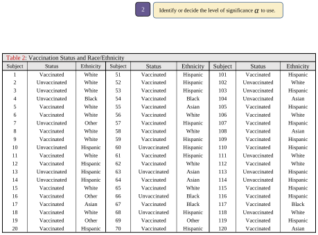
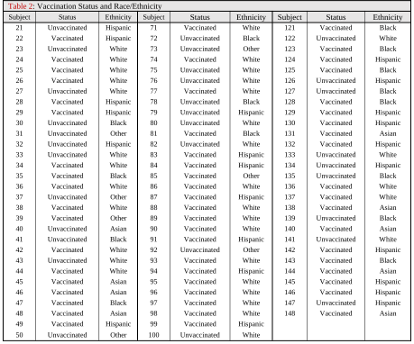
Table 2: Vaccination Status and Race/Ethnicity | ||||||||
|---|---|---|---|---|---|---|---|---|
Subject | Status | Ethnicity | Subject | Status | Ethnicity | Subject | Status | Ethnicity |
1 | Vaccinated | White | 51 | Vaccinated | Hispanic | 101 | Vaccinated | Hispanic |
2 | Unvaccinated | White | 52 | Vaccinated | Hispanic | 102 | Unvaccinated | White |
3 | Unvaccinated | White | 53 | Vaccinated | Hispanic | 103 | Unvaccinated | Hispanic |
4 | Unvaccinated | Black | 54 | Vaccinated | Black | 104 | Unvaccinated | Asian |
5 | Vaccinated | White | 55 | Vaccinated | Asian | 105 | Vaccinated | Hispanic |
6 | Vaccinated | White | 56 | Vaccinated | White | 106 | Vaccinated | White |
7 | Unvaccinated | Other | 57 | Vaccinated | Hispanic | 107 | Vaccinated | Hispanic |
8 | Vaccinated | White | 58 | Vaccinated | White | 108 | Vaccinated | Asian |
9 | Vaccinated | White | 59 | Vaccinated | Hispanic | 109 | Vaccinated | Hispanic |
10 | Unvaccinated | Hispanic | 60 | Unvaccinated | Hispanic | 110 | Vaccinated | Hispanic |
11 | Vaccinated | White | 61 | Vaccinated | Hispanic | 111 | Unvaccinated | White |
12 | Vaccinated | Hispanic | 62 | Vaccinated | White | 112 | Vaccinated | White |
13 | Unvaccinated | Hispanic | 63 | Unvaccinated | Asian | 113 | Unvaccinated | Hispanic |
14 | Unvaccinated | Hispanic | 64 | Vaccinated | Asian | 114 | Unvaccinated | Hispanic |
15 | Vaccinated | White | 65 | Vaccinated | White | 115 | Vaccinated | Hispanic |
16 | Vaccinated | Other | 66 | Unvaccinated | Black | 116 | Vaccinated | Hispanic |
17 | Vaccinated | Asian | 67 | Vaccinated | Black | 117 | Vaccinated | Black |
18 | Vaccinated | White | 68 | Unvaccinated | Hispanic | 118 | Unvaccinated | White |
19 | Vaccinated | Other | 69 | Vaccinated | Other | 119 | Vaccinated | Hispanic |
20 | Vaccinated | Hispanic | 70 | Vaccinated | Hispanic | 120 | Vaccinated | Asian |
21 | Unvaccinated | Hispanic | 71 | Vaccinated | White | 121 | Vaccinated | Black |
22 | Vaccinated | Hispanic | 72 | Unvaccinated | Black | 122 | Unvaccinated | White |
23 | Unvaccinated | White | 73 | Unvaccinated | Other | 123 | Vaccinated | Black |
24 | Vaccinated | White | 74 | Vaccinated | White | 124 | Vaccinated | Hispanic |
25 | Vaccinated | White | 75 | Unvaccinated | White | 125 | Vaccinated | Black |
26 | Vaccinated | White | 76 | Unvaccinated | White | 126 | Unvaccinated | Hispanic |
27 | Unvaccinated | White | 77 | Vaccinated | White | 127 | Unvaccinated | Black |
28 | Vaccinated | Hispanic | 78 | Unvaccinated | Black | 128 | Vaccinated | Black |
29 | Vaccinated | Hispanic | 79 | Unvaccinated | Hispanic | 129 | Vaccinated | Hispanic |
30 | Unvaccinated | Black | 80 | Unvaccinated | White | 130 | Vaccinated | Hispanic |
31 | Unvaccinated | Other | 81 | Vaccinated | Black | 131 | Vaccinated | Asian |
32 | Unvaccinated | Hispanic | 82 | Unvaccinated | White | 132 | Vaccinated | Hispanic |
33 | Unvaccinated | White | 83 | Vaccinated | Hispanic | 133 | Unvaccinated | White |
34 | Vaccinated | White | 84 | Vaccinated | Hispanic | 134 | Unvaccinated | Hispanic |
35 | Vaccinated | Black | 85 | Vaccinated | Other | 135 | Unvaccinated | Black |
36 | Vaccinated | White | 86 | Vaccinated | White | 136 | Vaccinated | White |
37 | Unvaccinated | Other | 87 | Vaccinated | Hispanic | 137 | Vaccinated | White |
38 | Vaccinated | White | 88 | Vaccinated | White | 138 | Vaccinated | Asian |
39 | Vaccinated | Other | 89 | Vaccinated | White | 139 | Unvaccinated | Black |
40 | Unvaccinated | Asian | 90 | Vaccinated | White | 140 | Vaccinated | Asian |
41 | Unvaccinated | Black | 91 | Vaccinated | Hispanic | 141 | Unvaccinated | White |
42 | Vaccinated | White | 92 | Unvaccinated | Other | 142 | Vaccinated | Hispanic |
43 | Unvaccinated | White | 93 | Vaccinated | White | 143 | Vaccinated | Black |
44 | Vaccinated | White | 94 | Vaccinated | Hispanic | 144 | Vaccinated | Asian |
45 | Vaccinated | Asian | 95 | Vaccinated | White | 145 | Vaccinated | Hispanic |
46 | Vaccinated | Asian | 96 | Vaccinated | White | 146 | Vaccinated | Hispanic |
47 | Vaccinated | Black | 97 | Vaccinated | White | 147 | Unvaccinated | Hispanic |
48 | Vaccinated | Asian | 98 | Vaccinated | White | 148 | Vaccinated | Asian |
49 | Vaccinated | Hispanic | 99 | Vaccinated | Hispanic | |||
50 | Unvaccinated | Other | 100 | Unvaccinated | White | |||
Step 3:We will treat this as a random sample, even though it was a student survey and was likely not truly randomized. It does meet the requirements for a binomial experiment. We still need to check that , using n = 148 and p = 0.78
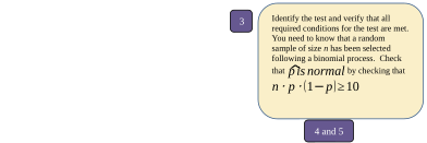
Since , the distribution of sampling proportions will have an approximately normal distribution.
Steps 4 and 5:
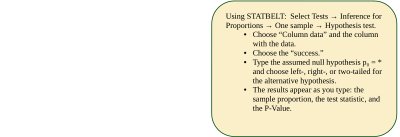
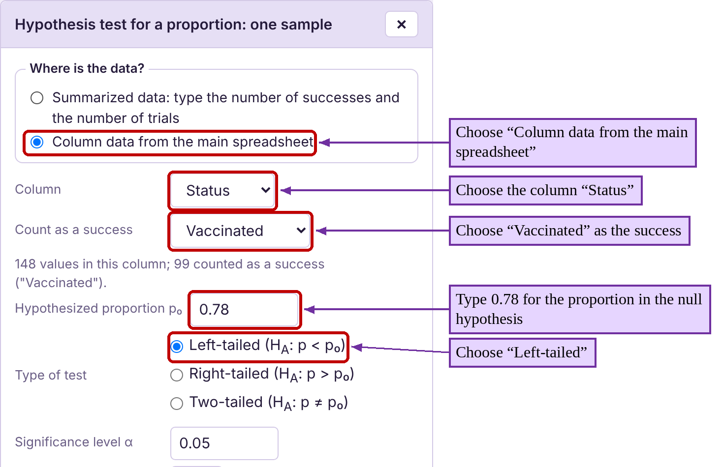
Open the vaccination data in STATBELT Utility with the link in the example. STATBELT opens with the columns “Status” and “Ethnicity” already loaded. Select Tests → Inference for Proportions → One sample → Hypothesis test.
Choose “Column data from the main spreadsheet” and the column “Status.” Choose “Vaccinated” as the success, since we are interested in the proportion who are vaccinated. Type 0.78 for p₀, the proportion in the null hypothesis. Since this is a left tailed test, choose “Left-tailed.”
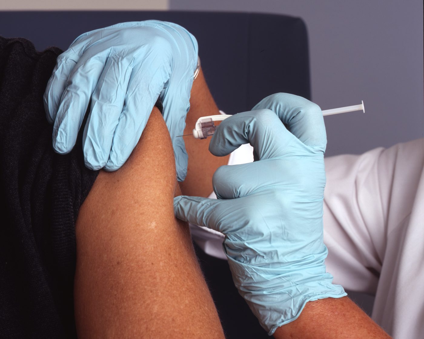
Photo by National Cancer Institute (opens in a new tab) on Unsplash (opens in a new tab)
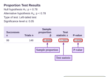
The output gives us the sample proportion vaccinated Americans in December 2021 as , or about 66.9%. The test statistic is -3.262, and P-Value = 0.0006.
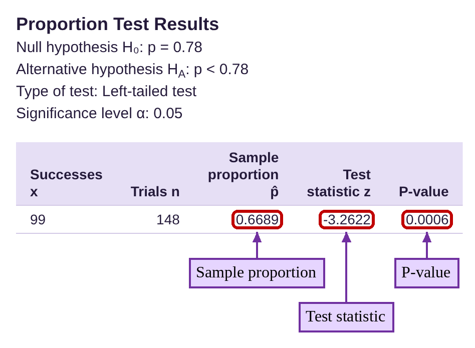
Step 6:Since the P-value = 0.0006 is less than , we reject the null hypothesis. There is statistical evidence to conclude that the proportion of Americans who had received at least one dose of a COVID-19 vaccine was lower in December 2021 that it was in July 2022.


In context, this means that there is about a 6 in 10,000 chance that this sample proportion (or lower) would occur in a sample of 148 individuals if the rate of vaccination in December 2021 was 78%, as it is reported to be today. Remember that the P-Value is the probability of a type 1 error. So, there is a 6 in 10,000 chance that we are rejecting the null hypothesis, even though it is true. For that reason, it seems logical to conclude that the rate was lower in December 2021.